A Brief Intro to Bayesian Inference for Accounting Research


Harm Schütt, Tilburg University

2023-10-05

Part 1
Why learn something about Bayesian Statistics?

  1. What is Bayesian statistics?

  2. What is it useful for?

What is Bayesian statistics? (oversimplified)


Frequentist: \(P(Data|Hypothesis)\)

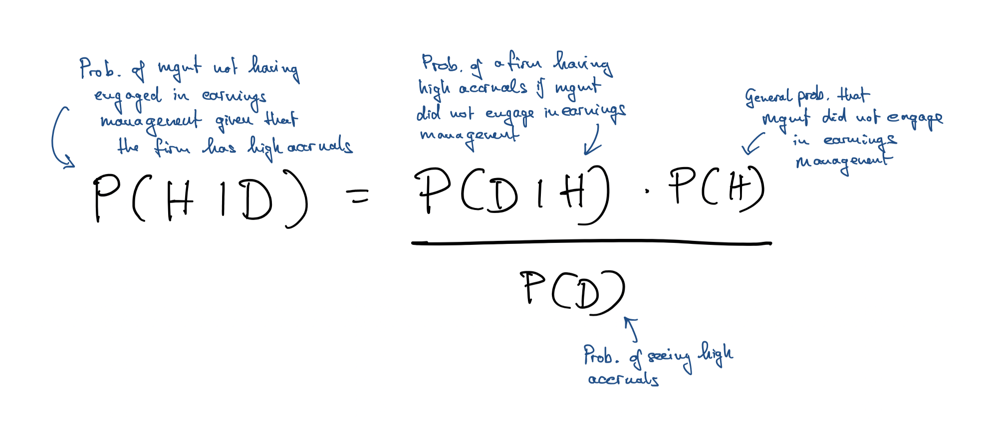
Bayesian: \(P(Hypothesis|Data)\)

\(P(H | D) = (P(D|H) * P(H)) / P(D)\) means updating


Example: Number of successful investments \(y \sim Binom(y|N,\theta)\)

Why learn a bit of Bayesian statistics?

Photo by Erik Mclean

Not because of the philosophical differences!

To better understand frequentist statistics

To add another tool to our workbench:

  • Sometimes the data is not informative enough
  • Priors and DGP helps encode additional information/assumptions
  • Useful for constructing finer measures and measuring latent constructs

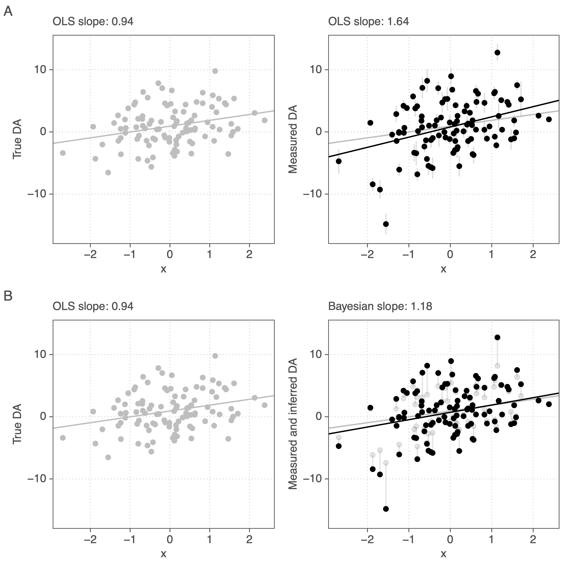
Example: Precise firm-level measures

\[R_{i,t} = a_i + b_i * X_{i,t} + u_{i,t}\]

Cross-learning the prior. Helps discipline noisy estimates

Example: Modeling uncertainty

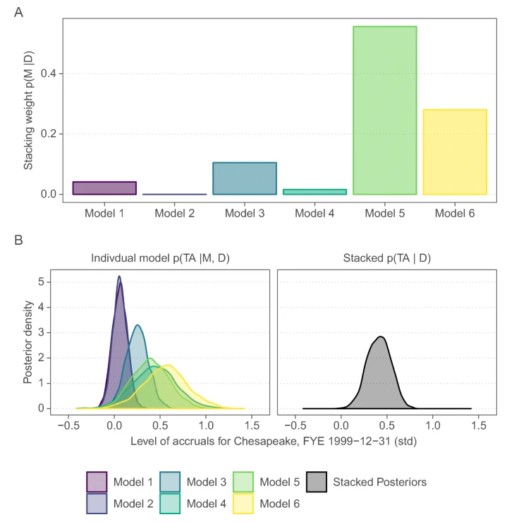
When we do not trust our models we should average. Increases power and reduce false positives in tests for opportunistic earnings management

Example: Modelling hidden dynamics (1)


How well do earnings reveal an unobserved true state of the firm?

Example: Modelling hidden dynamics (2)

Disclosures become more (less) frequent when investors’perception of the firm is worse (better) than the true profitability

Summary: Where does Bayes help?

  • Modeling heterogeneity. E.g., firm-level measures
  • Modeling uncertainty
  • Modeling latent constructs

Modeling a data-generating-process (incl. priors) allows us to include more information/assumptions into our analysis

Part 2
The Frequentist Baseline

  1. Data is random. The logic behind hypothesis tests.

  2. The importance of test power

  3. Overfitting is a serious issue

Some simulated datasets

  • Simulate 50 samples from: \(y = 1 + 2 \times x + u,\ u\sim N(0, 20)\).
  • \(x\) is only drawn once (not 50 times) from: \(x \sim N(0,1)\).
set.seed(888)
n_samples <- 50
n_obs <- 50
x_fix <- rnorm(n = n_obs, 0, 1)
gen_data <- function(n) tibble(u = rnorm(n, 0, 20), x = x_fix, y = 1 + 2 * x_fix + u)
samples <- tibble(id = 1:n_samples)
samples$data <- map(rep.int(n_obs, n_samples), gen_data)
samples
# A tibble: 50 × 2
      id data             
   <int> <list>           
 1     1 <tibble [50 × 3]>
 2     2 <tibble [50 × 3]>
 3     3 <tibble [50 × 3]>
 4     4 <tibble [50 × 3]>
 5     5 <tibble [50 × 3]>
 6     6 <tibble [50 × 3]>
 7     7 <tibble [50 × 3]>
 8     8 <tibble [50 × 3]>
 9     9 <tibble [50 × 3]>
10    10 <tibble [50 × 3]>
# ℹ 40 more rows
samples[[1, "data"]][[1]]
# A tibble: 50 × 3
        u      x      y
    <dbl>  <dbl>  <dbl>
 1  14.0  -1.95   11.1 
 2  -6.79 -1.54   -8.88
 3 -11.4   0.730  -8.90
 4  -3.22 -0.278  -2.78
 5  33.1  -1.66   30.8 
 6   6.45 -0.251   6.94
 7  14.2  -2.17   10.9 
 8  10.2   0.587  12.4 
 9   4.99  0.631   7.25
10 -20.9   1.10  -17.7 
# ℹ 40 more rows

Estimates vary across samples

\[y = a_0 + a_1 \times x + u\]

# A tibble: 50 × 5
      id     a0      a1 plabs       first_sample
   <int>  <dbl>   <dbl> <chr>       <fct>       
 1     1  0.760  4.38   (0.8,4.4)   1           
 2     2  1.76  -0.0400 (1.8,0)     0           
 3     3  6.46   0.738  (6.5,0.7)   0           
 4     4  3.20   0.561  (3.2,0.6)   0           
 5     5  0.328  5.24   (0.3,5.2)   0           
 6     6  0.786  6.17   (0.8,6.2)   0           
 7     7 -0.877 -1.58   (-0.9,-1.6) 0           
 8     8  2.18  -3.30   (2.2,-3.3)  0           
 9     9 -0.345  1.00   (-0.3,1)    0           
10    10 -0.545  3.49   (-0.5,3.5)  0           
# ℹ 40 more rows
  • Where is the variation in \(a_0\), \(a_1\) coming from?
  • Why? What are we trying to simulate?

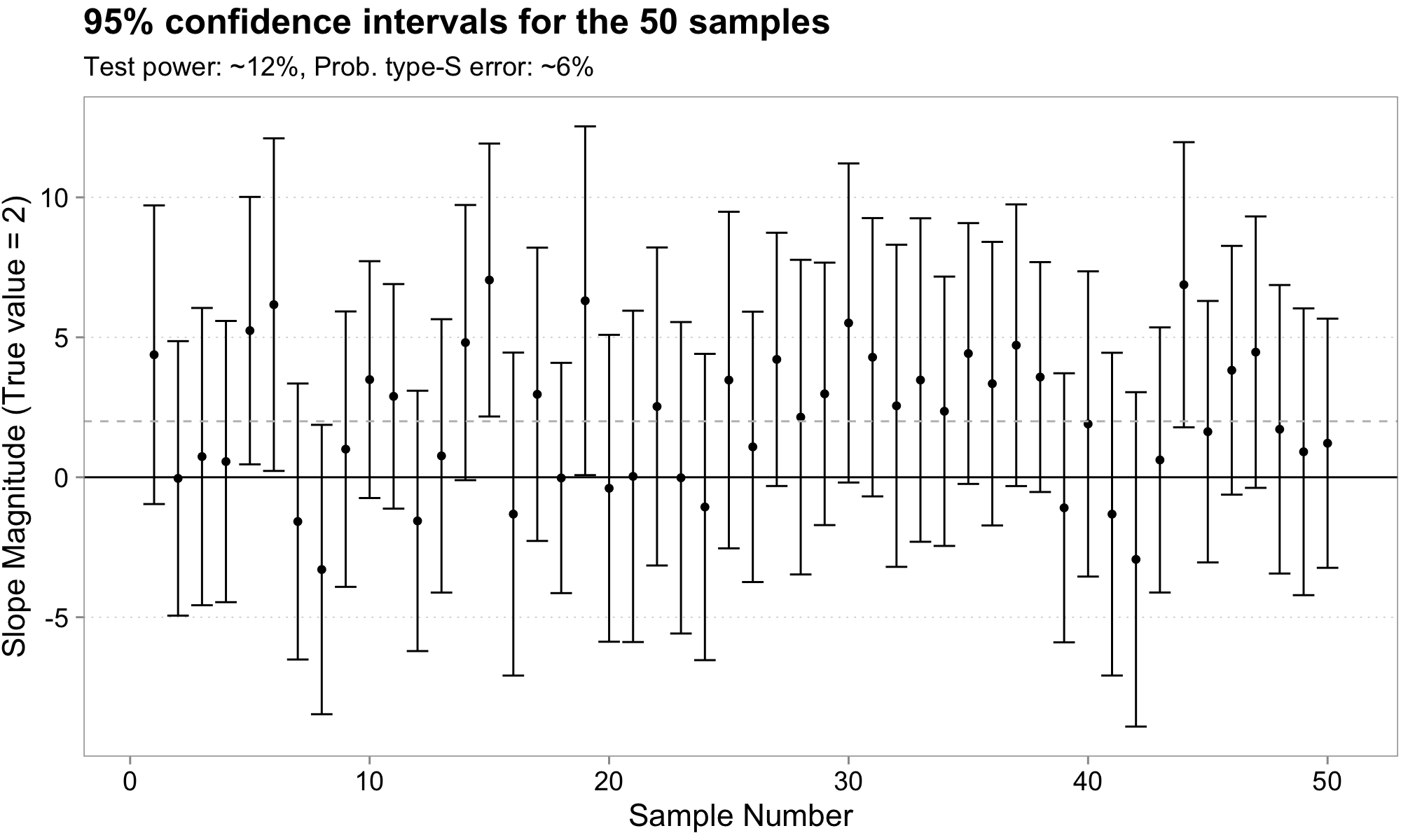
Unmeasured influences cause estimates to vary

\[y = 1 + 2 \times x + u ,\ u \sim N(0, 20),\ x\sim N(0,1)\]

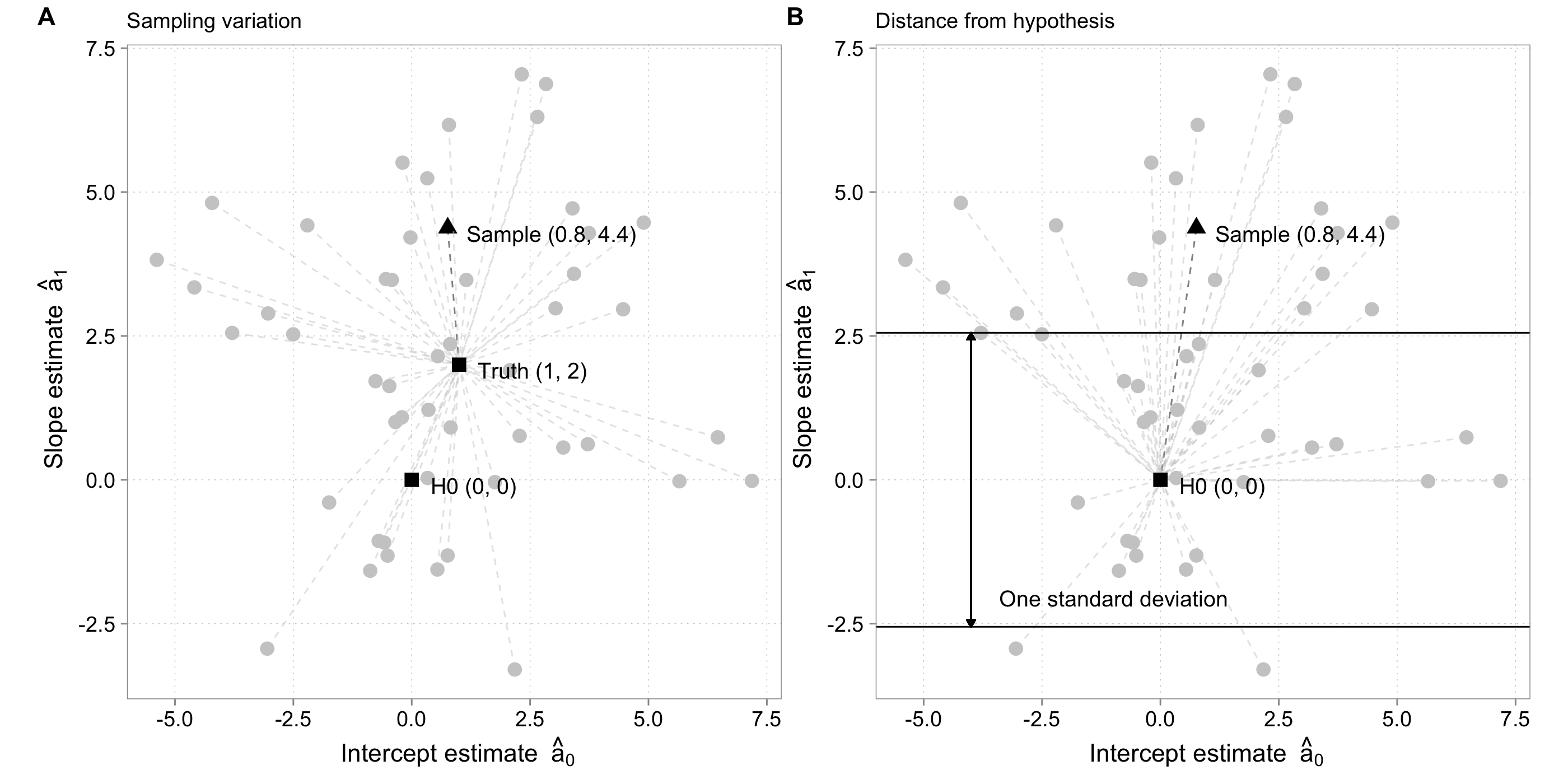
Hypothesis tests judge the data’s distance from \(H_0\)

Test logic:

  • Compute a “normalized distance” from \(H_0\) using S.E.
  • Figure out what distribution describes distance (assumptions)
  • Pick a threshold. When is an estimate considered too distant?
  • Too distant means: Unlikely to be generated under \(H_0\)

Normalization: S.E. depends on assumed behavior of unmeasured determinants (\(u\)) and \(N\)

Be careful interpreting coefficient magnitudes in low power situations

  • Coefficients very large for those intervals that do not include zero
  • Gets worse with less power (unexplained variance vs. N obs)
  • “That which does not destroy my statistical significance makes it stronger” fallacy

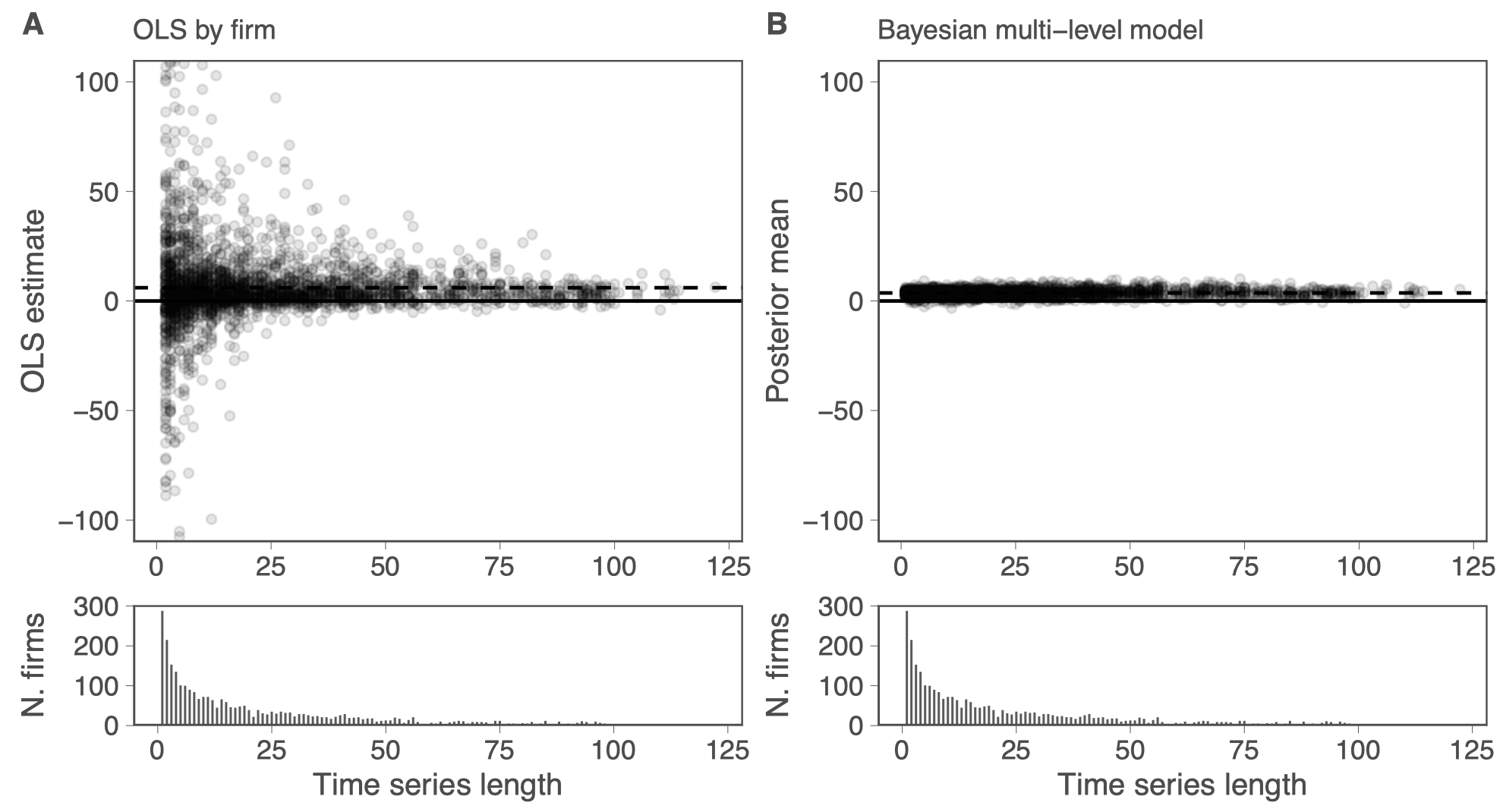
But my N is > 200.000 obs. Power is not an issue


Well … Let’s remember this picture

Effective N goes down quickly once we want to estimate heterogeneity in something we care about

And then there is overfitting…

Drawing 5 samples from \(y \sim N(-200 + 10 * x, (x+30)^2\)

Overfitting means we fitted sample idiosyncrasies

Differences in prediction errors (polynomial model MSE - linear model MSE)

Sample In-Sample MSE Difference Avg. Out-of-Sample MSE Difference
1 -8.5 -15.1
2 -1419.8 1770.0
3 -778.7 901.7
4 -2735.2 4602.0
5 -8.4 -15.1

Summary: Frequentist Statistics is great, but:

  • Right model: Significant estimates in low power situations are often way off
  • Model uncertainty: Overfitting can occur quite quickly

When we model heterogeneity or use complicated models, both issues become very important. Need to be dealt with.

Part 3
Using Bayesian inference to discipline the data

  1. Priors regularize, which combats overfitting and extreme estimates

  2. Priors can be learned from data

  3. A lot of extra information can be flexibly modeled

A simple Bayesian regression

First we define the DGP:

Likelihood \(P(D | H)\):

\[y = a_0 + a_1 * x + \epsilon, \,\,\,\, \epsilon \sim N(0, \sigma)\]

Coefficient priors \(P(a_k)\):

\[a_k \sim N(0, 100), \,\,\,k \in (0, 1)\]

Residual variance prior \(P(\sigma)\):

\[\sigma \sim Exponential(\frac{1}{21})\]

fit <- brm(
  y ~ x,
  data = sample1,
  chains = 4, cores = 4,
  prior = c(
    prior("normal(0, 100)", class = "b"),
    prior("normal(0, 100)", class = "Intercept"),
    prior("exponential(1.0/21.0)", class = "sigma")
    )
)

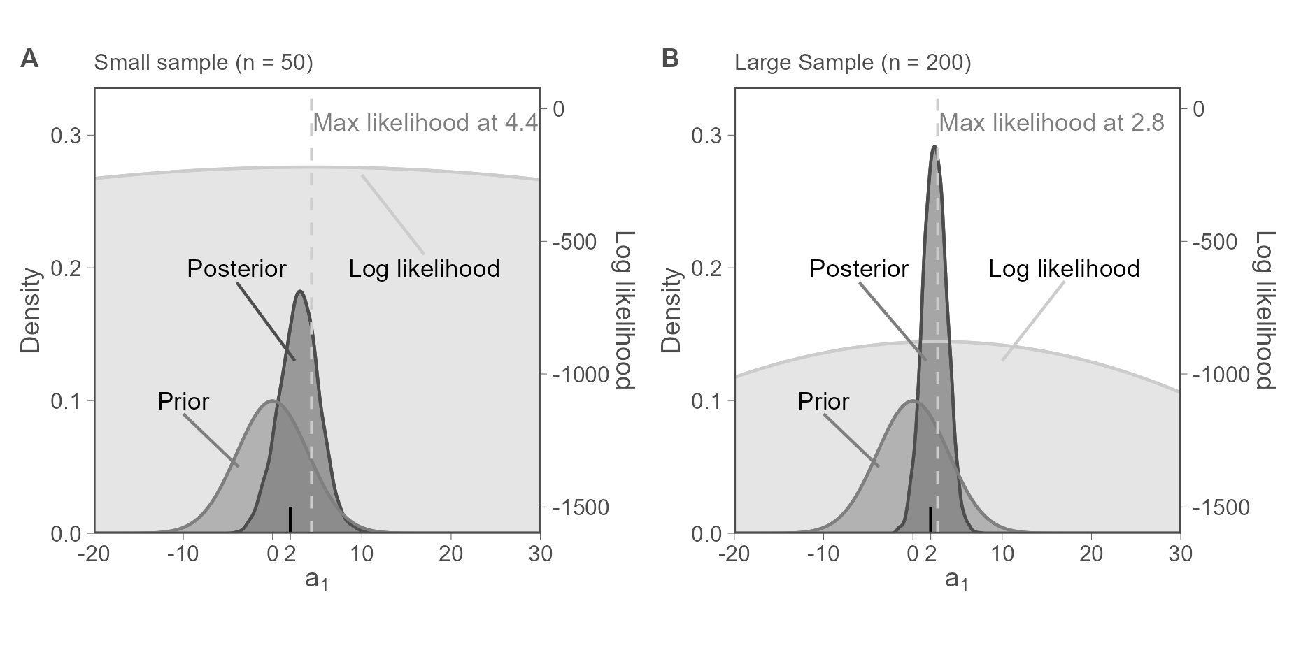
No additional information in the DGP


We basically get the same inference as with classic OLS

Imagine theory suggests that \(a_1\) cannot be large

Likelihood \(P(D | H)\):

\[y = a_0 + a_1 * x + \epsilon, \,\,\,\, \epsilon \sim N(0, \sigma)\]

Coefficient priors \(P(a_k)\):

\[a_0 \sim N(0, 100)\]

\[a_1 \sim N(0, 4)\]

Residual variance prior \(P(\sigma)\):

\[\sigma \sim Exponential(\frac{1}{21})\]

A weakly informative prior disciplines the model


Our posterior beliefs about \(a_1\) have moved closer to the truth.

Posteriors are bascially a weighted average of the likelihood and the prior


Assume \(y\sim N(\mu, \sigma^2)\) with known sigma and a prior for \(\mu \sim N(\mu_0, \sigma_0^2)\)

Then the posterior is a weighted average of the form:

\[P(\mu | y) \sim N\left(\frac{1}{\frac{1}{\sigma^2_0} + \frac{n}{\sigma^2}} * \left(\frac{1}{\sigma^2_0}*\mu_0 + \frac{n}{\sigma^2}*\frac{\sum^n y}{n}\right), \frac{1}{\frac{1}{\sigma^2_0} + \frac{n}{\sigma^2}}\right)\]

Priors have little weight when data is informative

An implication of the weighted average formula

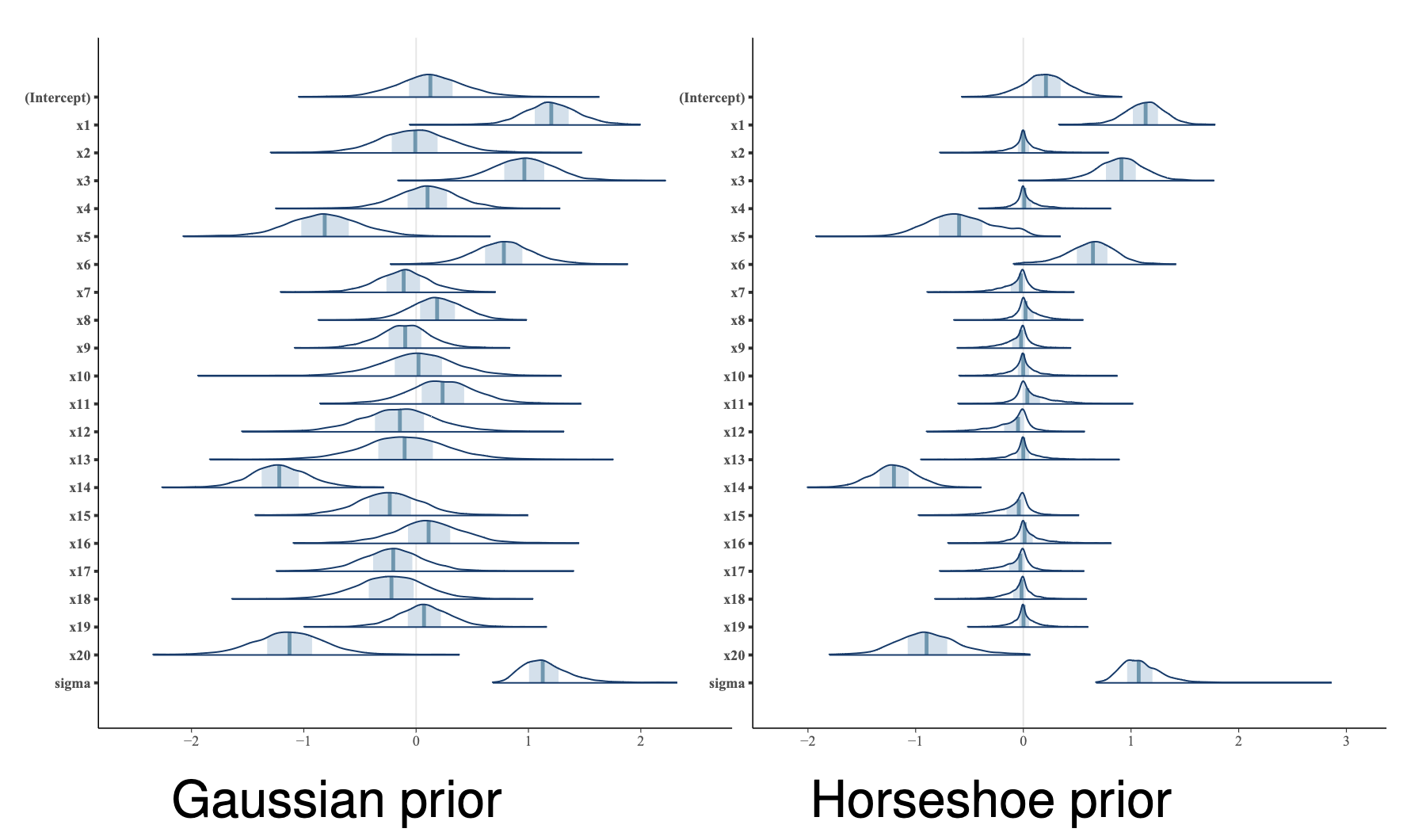
Priors help variable selection (think Lasso)

Especially relevant when:

  • Variables are noisy proxies
  • Variables are correlated (including interactions)

If we can assume that only a few covariates are effectively non-zero, we want sparse priors

Priors can be learned from the data

We can estimate priors, assuming that units come from the same distribution

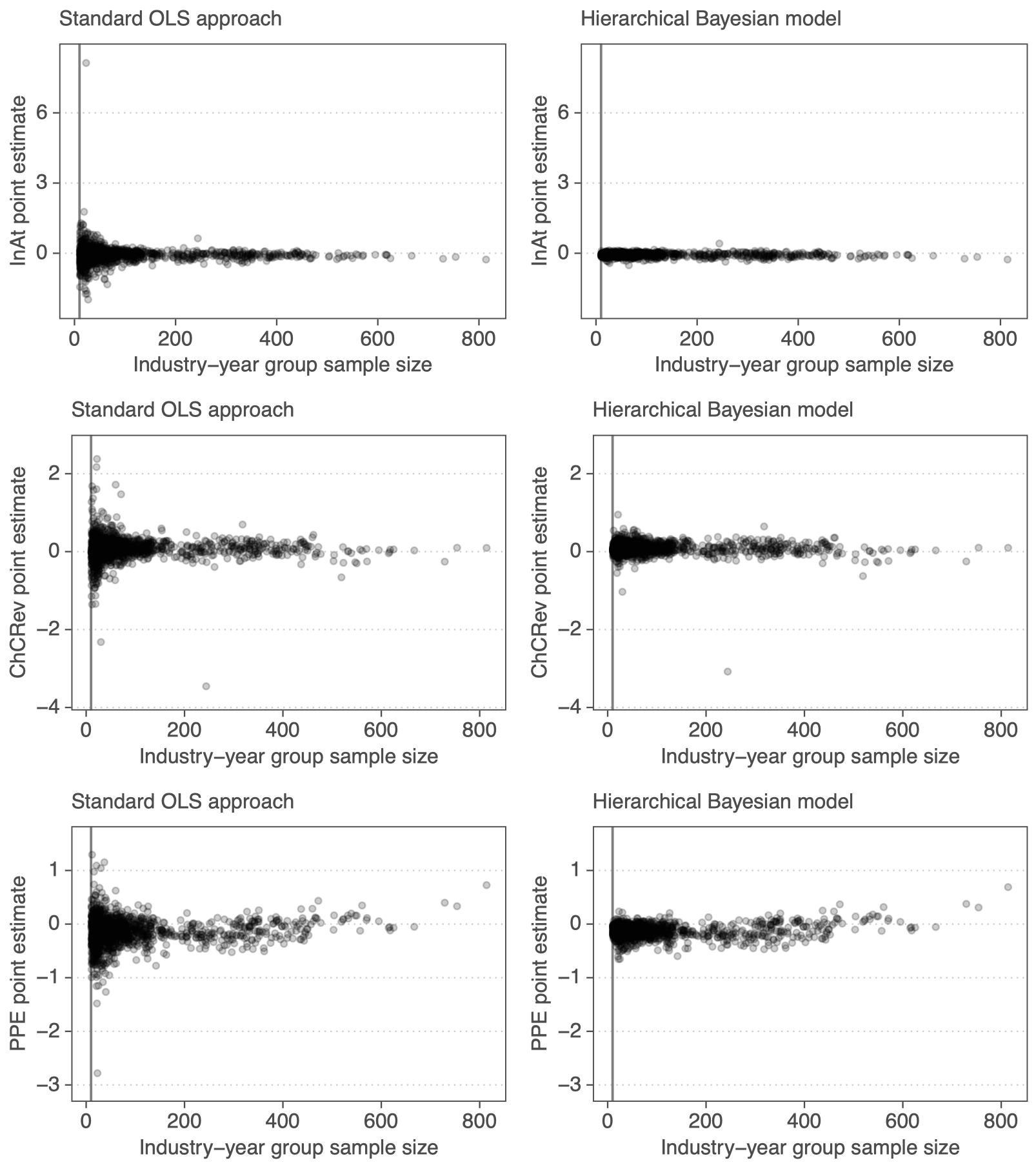
\[ \begin{align} TA_{ijt} & = \beta_{0,jt}InvAt_{ijt-1} + \beta_{1,jt}\triangle CRev_{ijt}\\\nonumber & + \beta_{2,jt}PPE_{ijt} \end{align} \]

Priors:

\[ \begin{eqnarray} \label{eq:priors} \begin{pmatrix} \beta_{0,j,t}\\ \beta_{1,j,t}\\ \beta_{2,j,t} \end{pmatrix} & \sim & N\left(\left(\begin{array}{c} \mu_0\\ \mu_1 \\ \mu_2 \end{array}\right),\left(\begin{array}{ccc} \sigma_{0} & \rho_{0,1} & \rho_{0,2} \\ \rho_{0,1} & \sigma_1 & \rho_{1,2} \\ \rho_{0,2} & \rho_{1,2} & \sigma_2 \end{array}\right)\right) \quad \forall j,t \end{eqnarray} \] Hyper-priors:

\[ \begin{align} \mu_d & \sim N\left(0, 2.5\right) \quad \sigma_d \sim Exp\left(1\right) \quad \forall d \nonumber \\ \rho & \sim LKJcorr(2) \end{align} \]

We want regularized measures + their uncertainty

Measurement error has serious consequences for our inferences

Priors can identify latent variables

We want to estimate newspaper slant. Assume that one needs room for interpretation to slant news:

\[ \begin{align} \textit{NrNegWords}_{i, j} & \sim \text{Binom}(N_{words}, p_{neg, i, j})\\ \nonumber \text{logit}(p_{neg, i, j}) & = \textit{RoomInt}_{j} \times {OutlNeg}_{i} + BadNews_{j} \end{align} \]

Model is not identified because: \(Room_j \times Outl_i = c*Room_j \times Outl_i/c\)

Priors (non-negative \(RoomInt\) + prior scale for \(Outl\)) identify it:

\[ \begin{eqnarray} \begin{pmatrix}log(Room_j)\\ News_j \end{pmatrix} & \sim & N\left(\left(\begin{array}{c} \mu_{LRoom}\\ \mu_{News} \end{array}\right),\left(\begin{array}{cc} \sigma_{LRoom} & \rho \\ \rho & \sigma_{News} \end{array}\right)\right)\\ \nonumber Outl_i & \sim & N(0, 1) \end{eqnarray} \]

Summary: Bayesian statistics is a useful tool because

  • Priors regularize, which combats overfitting and extreme estimates
  • Priors can be learned from data
  • A lot of extra information can be flexibly modeled

Bayesian statistics is not the only way to do all this. It’s advantage lies in its flexibility and in giving us powerful uncertainty measures for free.

Thank you for your attention

Next up: coding practice ;)