Part 1

Summary

This part discusses a simple example of loading and examining financial data from WRDS. We discuss how to use coding to explore, understand, and document the characteristics of your data. While doing so you will learn the basics tidyverse and collapse commands. We will finish with a rudimentary analysis of changes in firm size over time by creating the following plot:

Start: Load the necessary packages

Once R, RStudio, and the relevant R packages are installed we can start analyzing data. To load the data and start examining it, we want access to a few additional functions that are not in base R. The functions used in this chapter are contained in package collection called tidyverse. We also want to use some extra functionality in the {collapse} package. These packages contain very useful and popular extra functionality not included in base R. Anytime you want to load an R package for the extra functionality it brings, you type and execute a library function call:

Put your library statements, etc. at the top of each script. This makes it easier to see what packages are needed to run the code that follows
library(collapse)
collapse 1.9.6, see ?`collapse-package` or ?`collapse-documentation`

Attache Paket: 'collapse'
Das folgende Objekt ist maskiert 'package:stats':

    D
library(tidyverse)
── Attaching core tidyverse packages ──────────────────────── tidyverse 2.0.0 ──
✔ dplyr     1.1.3     ✔ readr     2.1.4
✔ forcats   1.0.0     ✔ stringr   1.5.0
✔ ggplot2   3.4.3     ✔ tibble    3.2.1
✔ lubridate 1.9.2     ✔ tidyr     1.3.0
✔ purrr     1.0.2     
── Conflicts ────────────────────────────────────────── tidyverse_conflicts() ──
✖ dplyr::filter()      masks stats::filter()
✖ lubridate::is.Date() masks collapse::is.Date()
✖ dplyr::lag()         masks stats::lag()
ℹ Use the conflicted package (<http://conflicted.r-lib.org/>) to force all conflicts to become errors

These two lines load the collapse package and the core tidyverse packages like ggplot2, dplyr, etc. It tells you in the message under “Attaching core tidyverse packages” exactly which packages it attached and which versions. It also tells you which functions from the loaded packages have a name conflict with functions in base R (or from other packages you might have loaded).

If you get an error there is no package called ‘tidyverse’, you’ll need to first install it, then run library() again.The command is

install.packages("tidyverse")

You only need to install a package once, but you need to load it every time you start a new session.

Once we have the packages loaded, we can start using their extra functionality. The tidyverse packages introduce an R coding framework that is slightly different from base R. Arguably, it is easier and still powerful. These days, it is probably the most common way of coding in R, which is why we chose to teach you using tidyverse mechanics and not pure base R. This does not mean that you cannot do what we do with standard R functions, but it is often clumsier.

Getting data

Because you will mostly encounter financial data in your professional life as well as the master program, our examples will be based on standard financial databases. This should help you a lot later on, for example when you start your replication study. Normally you would download this data from WRDS or access the data directly from a database. In the interest of time, we provide you with a raw dataset.

Loading data

Say we have downloaded some data from the Compustat North America file from WRDS and put it into a folder called data/. We labelled the file “ccm-raw-2023-08-08-csv”. That name is deliberate as it denotes that the file contains the raw, untouched data and shows the date it was downloaded.

The Compustat North America file contains some selected financial variables for publicly listed firms in North America. We want to load that file into R, so that we can examine it. The following code line does that:

ccm_raw <- read_csv("data/ccm-raw-2023-08-08-csv.zip")
Rows: 271143 Columns: 29
── Column specification ────────────────────────────────────────────────────────
Delimiter: ","
chr  (16): GVKEY, LINKPRIM, LIID, LINKTYPE, indfmt, consol, popsrc, datafmt,...
dbl  (12): LPERMNO, fyear, fyr, at, ceq, che, dlc, dltt, ib, oiadp, sale, exchg
date  (1): datadate

ℹ Use `spec()` to retrieve the full column specification for this data.
ℹ Specify the column types or set `show_col_types = FALSE` to quiet this message.

readr::read_csv is a function for—your guessed it—loading “.csv” files (csv: comma separated value).1 This line can be read from left to right as: “create an object called ccm_raw, assign (<-) to it the result of the function call read_csv()”. The result of read_csv is whatever that function does to its input. The input in this case is a file path in string form: “data/ccm-raw-2023-08-08-csv.zip”. Good function names tell you what the function does. In this case, it is pretty expressive: the function reads in a csv file. (Here, it actually reads in a zip file that contains a .csv file.) So what is the content of ccm_raw now? If you type the object name into the console and hit execute, you see that ccm_raw is a tibble, a type of data table.

When we first introduce a function, we will use a package::function notation (e.g., readr::read_csv) to point to the package the function is included in. So that you know what packages need to be loaded before you can run the code
ccm_raw
# A tibble: 271,143 × 29
   GVKEY  LINKPRIM LIID  LINKTYPE LPERMNO datadate   fyear indfmt consol popsrc
   <chr>  <chr>    <chr> <chr>      <dbl> <date>     <dbl> <chr>  <chr>  <chr> 
 1 001001 P        01    LU         10015 1983-12-31  1983 INDL   C      D     
 2 001001 P        01    LU         10015 1984-12-31  1984 INDL   C      D     
 3 001001 P        01    LU         10015 1985-12-31  1985 INDL   C      D     
 4 001003 C        01    LU         10031 1983-12-31  1983 INDL   C      D     
 5 001003 C        01    LU         10031 1984-12-31  1984 INDL   C      D     
 6 001003 C        01    LU         10031 1986-01-31  1985 INDL   C      D     
 7 001003 C        01    LU         10031 1987-01-31  1986 INDL   C      D     
 8 001003 C        01    LU         10031 1988-01-31  1987 INDL   C      D     
 9 001003 C        01    LU         10031 1989-01-31  1988 INDL   C      D     
10 001004 P        01    LU         54594 1981-05-31  1980 INDL   C      D     
# ℹ 271,133 more rows
# ℹ 19 more variables: datafmt <chr>, tic <chr>, cusip <chr>, conm <chr>,
#   curcd <chr>, fyr <dbl>, at <dbl>, ceq <dbl>, che <dbl>, dlc <dbl>,
#   dltt <dbl>, ib <dbl>, oiadp <dbl>, sale <dbl>, exchg <dbl>, costat <chr>,
#   fic <chr>, priusa <chr>, sic <chr>

Tibbles are the tidyverse versions of data tables. Similar to tables you are familiar with from Excel. They are also called data frames in many statistical programming languages. Data frames are the data container type you will encounter most. There are other container types, like matrix, which is a simpler data container that is mostly used for matrix algebra. We won’t spend time on those, because you’ll be mostly concerned with data in table form.2

ccm_raw <- rename(ccm_raw, 
                  gvkey = GVKEY, permno = LPERMNO,
                  liid = LIID, linktype = LINKTYPE, linkprim = LINKPRIM)

Adding labels to columns

This is not mandatory, but can make your life a lot easier. Especially if you get data with semi-cryptic names. Assigning labels to to columns will help you (and potential coauthors) later to remember what you are looking at. Some functions can also take advantage of labels. collapse::vlabels can be used to assign labels. You do so by assigning a “named vector” (using the concatenate c() function to create the vector) to vlabels(DATAFRAMENAME):

You can also just rename columns; give them more expressive names. For commercial datasets, we think it is better to keep the standard names for the raw data.
vlabels(ccm_raw) <- c( 
  # order must be the same as the columns:
  "gvkey" = "Standard and Poor's Identifier",
  "linkprim" = "Primary Link Marker",
  "liid" = "Security-level Identifier",
  "linktype" = "Link Type Code",
  "permno" = "Historical CRSP Identifier",
  "datadate" = "Fiscal Year-End Date",
  "fyear" = "Data Year - Fiscal",
  "indfmt" = "Industry Format",
  "consol" = "Consolidation Level",
  "popsrc" = "Population Source",
  "datafmt" = "Data Format",
  "tic" = "Ticker Symbol",
  "cusip" = "CUSIP",
  "conm" = "Company Name",
  "curcd" = "Currency",
  "fyr" = "Fiscal Year-End",
  "at" = "Assets - Total",
  "ceq" = "Common/Ordinary Equity - Total",
  "che" = "Cash and Short-Term Investments",
  "dlc" = "Debt in Current Liabilities - Total",
  "dltt" = "Long-Term Debt - Total",
  "ib" = "Income Before Extraordinary Items",
  "oiadp" = "Operating Income After Depreciation",
  "sale" = "Sales/Turnover (Net)",
  "exchg" = "Stock Exchange Code",
  "costat" = "Company Status",
  "fic" = "Foreign Incorporation Code",
  "priusa" = "PRIUSA -- Current Primary Issue Tag",
  "sic" = "Standard Industry Classification Code"
)

Examining data

Table meta data functions

When you typed ccm_raw, R did not print the full table. It tells you that there are 271,133 more rows and 19 more variables that you don’t see here. This printing behavior is mostly to save you from accidentally outputting huge datasets and freeze your machine. There are other functions to help you get a better overview of the data contained in the tibble. One is dplyr::glimpse

glimpse(ccm_raw)
Rows: 271,143
Columns: 29
$ gvkey    <chr> "001001", "001001", "001001", "001003", "001003", "001003", "…
$ linkprim <chr> "P", "P", "P", "C", "C", "C", "C", "C", "C", "P", "P", "P", "…
$ liid     <chr> "01", "01", "01", "01", "01", "01", "01", "01", "01", "01", "…
$ linktype <chr> "LU", "LU", "LU", "LU", "LU", "LU", "LU", "LU", "LU", "LU", "…
$ permno   <dbl> 10015, 10015, 10015, 10031, 10031, 10031, 10031, 10031, 10031…
$ datadate <date> 1983-12-31, 1984-12-31, 1985-12-31, 1983-12-31, 1984-12-31, …
$ fyear    <dbl> 1983, 1984, 1985, 1983, 1984, 1985, 1986, 1987, 1988, 1980, 1…
$ indfmt   <chr> "INDL", "INDL", "INDL", "INDL", "INDL", "INDL", "INDL", "INDL…
$ consol   <chr> "C", "C", "C", "C", "C", "C", "C", "C", "C", "C", "C", "C", "…
$ popsrc   <chr> "D", "D", "D", "D", "D", "D", "D", "D", "D", "D", "D", "D", "…
$ datafmt  <chr> "STD", "STD", "STD", "STD", "STD", "STD", "STD", "STD", "STD"…
$ tic      <chr> "AMFD.", "AMFD.", "AMFD.", "ANTQ", "ANTQ", "ANTQ", "ANTQ", "A…
$ cusip    <chr> "000165100", "000165100", "000165100", "000354100", "00035410…
$ conm     <chr> "A & M FOOD SERVICES INC", "A & M FOOD SERVICES INC", "A & M …
$ curcd    <chr> "USD", "USD", "USD", "USD", "USD", "USD", "USD", "USD", "USD"…
$ fyr      <dbl> 12, 12, 12, 12, 12, 1, 1, 1, 1, 5, 5, 5, 5, 5, 5, 5, 5, 5, 5,…
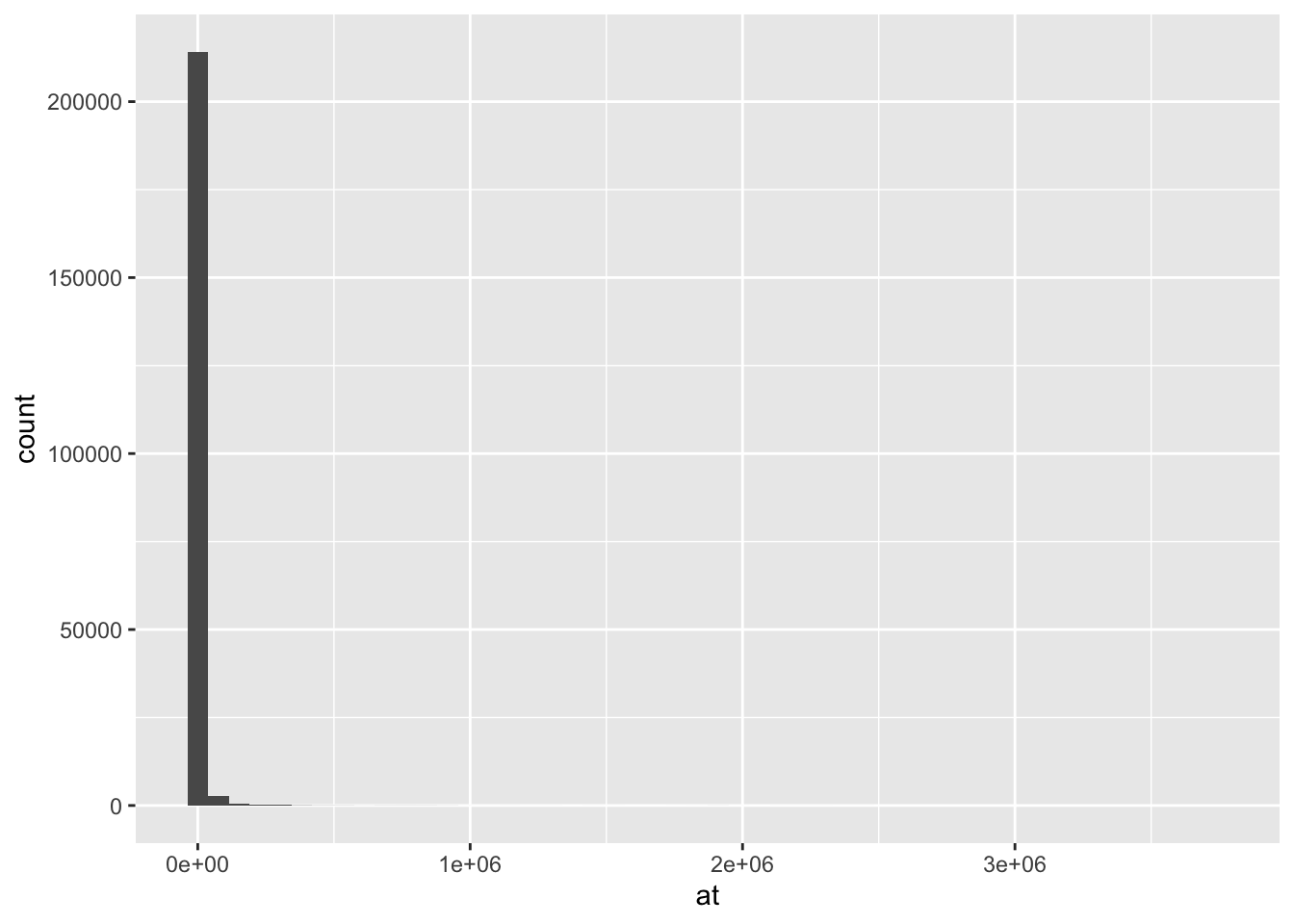
$ at       <dbl> 14.080, 16.267, 39.495, 8.529, 8.241, 13.990, 14.586, 16.042,…
$ ceq      <dbl> 7.823, 8.962, 13.014, 6.095, 6.482, 6.665, 7.458, 7.643, -0.1…
$ che      <dbl> 4.280, 1.986, 2.787, 2.023, 0.844, 0.005, 0.241, 0.475, 0.302…
$ dlc      <dbl> 0.520, 0.597, 8.336, 0.250, 0.350, 0.018, 0.013, 0.030, 7.626…
$ dltt     <dbl> 4.344, 4.181, 11.908, 0.950, 0.600, 4.682, 3.750, 5.478, 0.10…
$ ib       <dbl> 1.135, 1.138, 2.576, 1.050, 0.387, 0.236, 0.793, -0.525, -7.8…
$ oiadp    <dbl> 1.697, 1.892, 5.238, 2.089, 0.732, 0.658, 1.933, -0.405, -4.3…
$ sale     <dbl> 25.395, 32.007, 53.798, 13.793, 13.829, 24.189, 36.308, 37.35…
$ exchg    <dbl> 14, 14, 14, 19, 19, 19, 19, 19, 19, 11, 11, 11, 11, 11, 11, 1…
$ costat   <chr> "I", "I", "I", "I", "I", "I", "I", "I", "I", "A", "A", "A", "…
$ fic      <chr> "USA", "USA", "USA", "USA", "USA", "USA", "USA", "USA", "USA"…
$ priusa   <chr> "01", "01", "01", "01", "01", "01", "01", "01", "01", "01", "…
$ sic      <chr> "5812", "5812", "5812", "5712", "5712", "5712", "5712", "5712…

glimpse just shows you in compact form: 1) the number of rows, 2) the number of columns, 3) all column names, 4) column types, and 5) the first values in each column in the table

An alternative to glimpse that does not rely on dplyr being loaded in is the base R function: base::str. But it is usually less clean, so we prefer glimpse.

Data viewers

If you use RStudio or VScode as your IDE (integrated development environment), then you can also view tibbles/data.frames/data.tables in a viewer. In RStudio, you can click on the tibble name “ccm_raw” in the environment pane, hitting the F2-key if the cursor is on the “ccm_raw” also opens the data viewer. Or you can use the function tibble::view to start the data viewer.

view(ccm_raw)

Getting a structured overview

When dealing with large datasets, looking at the data viewer will not be enough. One of the first things you should do is to get a better feeling for the data you are dealing with. If you want to get a glimpse of what countries are in this dataset, you cannot just browse through 300,000 rows. It will take too long and it is easy to miss rarely occurring patterns.

Things like examining the distinct values in a column help you a lot in better understanding your data. You can use the collapse::fndistinct function to check the number of distinct values per column

fndistinct(ccm_raw)
   gvkey linkprim     liid linktype   permno datadate    fyear   indfmt 
   25614        4       23        2    26099      518       44        1 
  consol   popsrc  datafmt      tic    cusip     conm    curcd      fyr 
       1        1        1    25613    25614    25612        2       12 
      at      ceq      che      dlc     dltt       ib    oiadp     sale 
  203359   176724   113664    70320   117375   118348   130310   185004 
   exchg   costat      fic   priusa      sic 
      15        2       64       23      449 

There are a few columns with just one distinct value. We don’t need those anymore. They were used to filter the raw data. In case you do not know/remember what those columns were, look at the labels.

1ccm_raw |>
2  select(indfmt, consol, popsrc, datafmt) |>
3  namlab()
1
Start with the ccm_raw dataset
2
Select four columns, throw the rest away (using dplyr::select)
3
Call namlabon the reduced tibble to see the column labels for the selected labels
  Variable               Label
1   indfmt     Industry Format
2   consol Consolidation Level
3   popsrc   Population Source
4  datafmt         Data Format
ccm_raw |>                                    
  select(indfmt, consol, popsrc, datafmt) |>  
1  funique()
1
collapse::funique shows only unique combinations in a data frame.
# A tibble: 1 × 4
  indfmt consol popsrc datafmt
  <chr>  <chr>  <chr>  <chr>  
1 INDL   C      D      STD    

Above, we used what is called a pipe operator |>. It allows us to chain together a sequence of steps. When you see a |>, it means “take the result of what is left of |> and put it as the first input to what is right of |>.

Back to the topic at hand, we do not need the columns: indfmt, consol, popsrc, datafmt. Let us get rid of them. We do so by generating a new dataset, which we call ccm and using a “negative” select call.

We like to keep the raw data untouched when filtering and cleaning data
ccm <- 
  ccm_raw |> 
  select(-indfmt, -consol, -popsrc, -datafmt) 

Examining individual columns

You would usually spend some more time understanding the data. For example, what about those with 2 values? We can use collapse::descr to provide some descriptive statistics. Notice how it also uses the labels we provided before.

ccm |> 
  select(curcd, costat) |> 
  descr()
Dataset: costat, 2 Variables, N = 271143
--------------------------------------------------------------------------------
curcd (character): Currency
Statistics (0% NAs)
       N  Ndist
  271141      2
Table
       Freq   Perc
USD  266735  98.38
CAD    4406   1.62
--------------------------------------------------------------------------------
costat (character): Company Status
Statistics
       N  Ndist
  271143      2
Table
     Freq   Perc
I  162350  59.88
A  108793  40.12
--------------------------------------------------------------------------------

Depending on how we define our setting, we might want to get rid of those financials in Canadian dollars curcd == "CAD". costatshows that 60% of our sample has the inactive status.

We can also call descr on single columns using $ to select a single column:

descr(ccm$fic)
Dataset: fic, 1 Variables, N = 271143
--------------------------------------------------------------------------------
fic (character): Foreign Incorporation Code
Statistics
       N  Ndist
  271143     64
Table
                 Freq   Perc
USA            241894  89.21
CAN              7703   2.84
CYM              2781   1.03
ISR              2418   0.89
GBR              2195   0.81
BMU              1806   0.67
IRL              1070   0.39
JPN               973   0.36
NLD               868   0.32
VGB               783   0.29
MHL               656   0.24
MEX               634   0.23
AUS               537   0.20
FRA               512   0.19
... 50 Others    6313   2.33

Summary of Table Frequencies
   Min. 1st Qu.  Median    Mean 3rd Qu.    Max. 
      3      31     130    4237     373  241894 
--------------------------------------------------------------------------------

There are 69 different countries of incorporation in this dataset. Most incorporated in the USA. We learn something interesting about the dataset. Not all firms in the North America Dataset are located in North America. Most firm-year obs are associated with USA incorporation. Some are incorporated in Canada, the next most often occurring is Cayman islands. Depending on our research question, we might want to restrict our sample only to firms incorporated in the US. Before making that call, however, we might want to explore the data a bit more.

We see that some observations are from firms incorporated in the Netherlands. Let us extract a sample of names of those companies.

1ccm |>
2  filter(fic == "NLD") |>
3  pull(conm) |>
4  unique() |>
5  head(20)
1
Start with the table ccm
2
Reduce the table to only rows with fic equaling (==) “NLD”
3
dplyr::pull extracts the “conm” column from the reduce table into a vector
4
Reduce to only unique values in the vector
5
Show the first 20 values in the vector
 [1] "ASM INTERNATIONAL NV"         "KLM-ROYAL DUTCH AIRLINES"    
 [3] "OCE NV"                       "KONINKLIJKE PHILIPS NV"      
 [5] "ROYAL DUTCH PETROLEUM NV"     "AUSIMONT NV"                 
 [7] "FIAT CHRYSLER AUTOMOBILES NV" "AKZO NOBEL NV"               
 [9] "ABN-AMRO HOLDINGS NV"         "AEGON NV"                    
[11] "ING GROEP NV"                 "FRANK'S INTL NV"             
[13] "PROSENSA HOLDING NV"          "POLYGRAM NV"                 
[15] "PATHEON NV"                   "MOBILEYE NV"                 
[17] "CNOVA NV"                     "PROQR THERAPEUTICS NV"       
[19] "AFFIMED NV"                   "MEMOREX TELEX NV  -ADR"      

The NLD firms are likely larger internationals that are listed on one of the US exchanges in some form, so that they have to file with the SEC (Companies listed on a US exchange must file financial statements with the SEC). Let’s look at ASM for example:

1ccm |>
2  filter(conm == "ASM INTERNATIONAL NV") |>
3  select(tic, cusip, conm, curcd, exchg) |>
4  distinct()
1
Start with the table ccm
2
Reduce the table to only rows with conm equaling (==) “ASM INTERNATIONAL NV”
3
Reduce the reduced table further to only contain the columns tic, cusip, conm, curcd, exchg
4
dplyr::distinctdrops all repeating rows in the reduced table (could have also used funique)
# A tibble: 1 × 5
  tic   cusip     conm                 curcd exchg
  <chr> <chr>     <chr>                <chr> <dbl>
1 ASMIY N07045102 ASM INTERNATIONAL NV USD      19

As the example above shows: dplyr::select and dplyr::filter are two fundamental slicing and indexing functions. filter is for rows and selectis for columns.

The purpose here was to examine what ticker, currency, and stock exchange code ASM is associated with. We also want to check whether there is more than one combination of values for these five columns (there is not). For example, ASM is in our sample for more than one year and it might have changed its ticker over time, etc.). We see that ASM has a ticker and an exchg code of 19, which means “Other-OTC” per the compustat data guide. These can include international filers. In fact, most of the observations fall into category 19 (another one, 14, is NASDAQ). Depending on the intended sample—US firms or firms listed in the US—we might want to exclude them.

Ensure one observation per unit of analysis

When you perform analyses, it is important that you are clear what your unit of analysis is. Let’s say that our unit of analysis is a firm-fiscal year. In that case, we need to check whether we have one observation per unit of analysis.

We can do this we simple counts.dplyr::count is a handy function for this. count, as the name suggests, counts how often a value of a set of variables occurs in the dataset. The first input you provide is the dataset, the next inputs are the column names to base the count on:

ccm |> 
1  count(gvkey, datadate) |>
2  head()
1
Count how many observations exist for each unique gvkey x datadate combination
2
Show the first six observations in the resulting tibble
# A tibble: 6 × 3
  gvkey  datadate       n
  <chr>  <date>     <int>
1 001001 1983-12-31     1
2 001001 1984-12-31     1
3 001001 1985-12-31     1
4 001003 1983-12-31     1
5 001003 1984-12-31     1
6 001003 1986-01-31     1

For example, the combination gvkey 001001 x date 1983-12-31 occurs exactly once in the datset ccm. We can combine two count calls to see whether we have anything to worry about:

ccm |> 
1  count(gvkey, datadate, name = "firm_year") |>
2  count(firm_year)
1
Count how many observations exist for each unique gvkey x datadate combination. Call the count column “firm_year”
2
Count how often each value of the “firm_year” column occurs
# A tibble: 3 × 2
  firm_year      n
      <int>  <int>
1         1 265776
2         2   2607
3         3     51

As you can see, there are a few gvkey x datadate combinations that occur twice, some even three times. Why is this happening? Let write some code to figure it out.

ccm_test <- ccm |> 
1  add_count(gvkey, datadate, name = "n_same_firm_year") |>
2  filter(n_same_firm_year > 1)
1
dplyr::add_count counts the number of rows with a specific gvkey x datadate value and adds that value to the rows with the respective gvkey x datadate value
2
Next we filter to only keep rows with a count higher than 1

Let’s look at the result and limit our output to only some selected columns and ten rows:

ccm_test |> 
  select(gvkey, permno, datadate, liid, linkprim, linktype, exchg) |> 
  head(10)
# A tibble: 10 × 7
   gvkey  permno datadate   liid  linkprim linktype exchg
   <chr>   <dbl> <date>     <chr> <chr>    <chr>    <dbl>
 1 001076  10517 1993-03-31 01    J        LC          11
 2 001076  78049 1993-03-31 02    P        LC          11
 3 001076  78049 1994-03-31 02    P        LC          11
 4 001076  10517 1994-03-31 01    J        LC          11
 5 001076  10517 1995-03-31 01    J        LC          11
 6 001076  78049 1995-03-31 02    P        LC          11
 7 001076  78049 1995-12-31 02    P        LC          11
 8 001076  10517 1995-12-31 01    J        LC          11
 9 001076  10517 1996-12-31 01    J        LC          11
10 001076  78049 1996-12-31 02    P        LC          11

From the output we can see that the reason is that this dataset has another company identifier (permno) merged to it already. This is the identifier we will need in the second part to merge stock return data to this sample. It can happen that one gvkey is associated with more than one permno. Sometimes there are primary and secondary links.

We decided that our unit of analysis is firm-year, not security-year. Hence we only want one unique observation per firm-year. For that, we will need to do some filtering. Let us reduce the data to rows that either are a unique gvkey x datadate combination, or are labelled as primary link between compustat and crsp (which we will need later to join return data on it). We will also filter to companies incorporated in the US. (e.g., as we would want to if we look at some US-GAAP specific analysis).

ccm_unique <- ccm |> 
1  add_count(gvkey, datadate, name = "n_same_firm_year") |>
  filter(             
2    n_same_firm_year == 1 | linkprim == "P",  # "|" means "or"
3    fic %in% c("USA")
  ) |>   
4  select(-n_same_firm_year)
1
Count how many observations exist for each unique gvkey x datadate combination. Call the count column “firm_year”
2
Keep rows with either n_same_firm_year == 1 or linkprim == “P”
3
Keep rows with fic in a list of values (“USA”)
4
Delete the column “n_same_firm_year”

We should now have one observation per gvkey x datadate unit of analysis. Let us double-check whether it is indeed the case.

ccm_unique |> 
  count(gvkey, datadate, name = "firm_year") |> 
  count(firm_year)
# A tibble: 1 × 2
  firm_year      n
      <int>  <int>
1         1 239192

We will leave it at that for now and save the result.

Saving datasets

You can save datasets to many different formats, e.g., back to .csv, to Stata or SAS files, excel files, and many many more. There is an R package for almost all file formats you might need. If you share data and don’t mind large files, csv is not a bad choice (e.g., using readr::write_csv). Do not save datsets to excel! Excel files have a row limit that is often exceeded and the chance that data formats and similar things get garbled is just too high. ({writexl} is a package including functions for writing excel files. {readxl} for reading).

R also has a way store datasets into binary format. These files are called .rds files. They are reasonably fast and compact, so not a bad choice for saving intermediate output that is not supposed to be stored permanently. We will use it now.

saveRDS(ccm_unique, "data/ccm-unique.rds")
# readRDS for reading the file in again

We will continue preparing the sample in the second part of the workshop “Transforming Data”.

Plotting to understand data

A good plotting library is an incredibly powerful tool to not only present results but also to explore and understand data. See for example the BBC Visual and Data Journalism cookbook for R graphics for some great examples of good plots. In our case, we wan to get a better feeling for how the distribution of firm size in our dataset.

We could start with a simple histogram

ccm_unique |> 
1  drop_na(at) |>
2  ggplot(aes(x = at)) +
3  geom_histogram(bins = 50)
1
Drop all rows with missing values of at (assets total) from the data frame
2
Create a plotting canvas with the x axis being mapped to at
3
Draw a histogram on the plot canvas using 50 bins

Unfortunately, we do not see much here. The reason is the extremely skewed distribution of variables like total assets, sales, household income. There is always a “Apple Inc.” that is so much larger, or a “Jeff Bezoz” that is so much richer than everyone else. For variables that can only have positive values, taking the logarithm can yield in a much easier visualization. But we need a to be a bit careful with our log-taking. If we have negative values, the log() function will produce missing values and if we take the log of zero we get “negative infinity” as a result

ccm_unique |> 
1  mutate(Size = log(at)) |>
2  select(at, Size) |>
3  qsu()
1
Mutate the data by taking the log of at and storing the result into a new column named “Size”
2
Only keep the columns at and Size. Drop all other columns
3
collapse:qsu computes a quick summary (qsu)
           N       Mean          SD   Min       Max
at    218211  4761.9387  47680.2673     0  3'743567
Size  218211          -           -  -Inf   15.1355

The -Inf is a problem when plotting so we filter it out before

ccm_unique |> 
1  mutate(Size = log(at)) |>
2  filter(is.finite(Size)) |>
3  ggplot(aes(x = Size)) +
4  geom_histogram(bins = 50)
1
Mutate the data by taking the log of at and storing the result into a new column named “Size”
2
Drop all rows with infinite values of Size from the data frame
3
Create a plotting canvas with the x axis being mapped to Size
4
Draw a histogram on the plot canvas using 50 bins

This looks much better. However, this is the distribution over all years in our sample. It might hide interesting patterns in the data. We could take a look at how the data changed over time. There is multiple ways we could try to visualize and explore such changes. Here is one. For this we need a third extra package called {ggrides}

library(ggridges)

If you are surprised that you need an yet another package to run the code, you should be. As we said above, this is bad coding practice. Put all your library calls always at the top of your scripts, so that everyone can always see what is required to run all code. ggridges contains functions to plot so-called ridge plots. We will use ggridges::geom_density_ridges for that.

1fig1 <-
  ccm_unique |>                                          
2  mutate(Size = log(at)) |>
  filter(                                                  
3    is.finite(Size),
4    !is.na(fyear) & fyear < 2023
  ) |> 
5  ggplot(aes(x = Size, y = as.factor(fyear))) +
6  geom_density_ridges(
    scale = 5, 
    fill = "coral", color = "black",
    alpha = 0.2, 
    rel_min_height = 0.005
  ) +
7  geom_vline(xintercept = 5, color = "grey30") +
8  scale_y_discrete(expand = c(0.01, 0)) +
9  scale_x_continuous(expand = c(0.01, 0)) +
10  theme_light() +
11  theme(panel.grid.minor = element_blank()) +
12  labs(
    y = "Fiscal Year",
    x = "Firm Size (log of total assets)",
    title = "Listed firms are much bigger today",
    subtitle = "Change in firm size distribution over time",
    caption = "Source: Compustat North America data (1980 - 2022). Not adjusted for inflation"
  )
1
Store the result of the computation into variable called fig1
2
Mutate the data by taking the log of at and storing the result into a new column named “Size”
3
Drop all rows with infinite values of Size from the data frame
4
Drop all rows with missing fiscal year (fyear) and fyear greater equal 2023
5
Create a plotting canvas with the x axis being mapped to Size and the y axis to fyear where fyear is transformed from an integer variable to a factor before. (A quirk of ggridges makes this necessary)
6
Draw a ridge plot on the plot canvas using a certain parameter configuration
7
Add a guiding vertical line that intersects the x axis at 5.
8
Reduce the padding around the x axis (The default padding is to much for my taste)
9
Reduce the padding around the y axis
10
Switch the standard grey theme to a lighter theme
11
Remove some unnecessary gridlines
12
Add annotations to finalize the plot

We have stored the plot into a variable called fig1 instead of plotting it directly. This is useful for post-processing, saving, etc. Here is the plot in fig1

fig1
Picking joint bandwidth of 0.361

And here is how to save it to disk in .png format (good for websites)

ggsave("size-by-year.png", fig1, width = 7, height = 7, units = "in")
Picking joint bandwidth of 0.361

Footnotes

  1. These are essentially text files that you could open in a text editor to look at the values. They have the advantage that most programs can read them (because they are text files). The disadvantage is that they usually take more disk space and take longer to read. That is something you will only notice with big files though.↩︎

  2. Base R also has a data.frame type, of which tibble is a derivative. There are also others, like data.table (which we won’t cover, even though it is awesome. It is advanced stuff). Except for data.table, they are mostly interchangeable.↩︎