Posts > Teaching > P/E and other valuation multiples
P/E and other valuation multiples
This is just a short note to make the code for the plots from week 7 of the FSA lecture available for those of you who wanted to play around with it.
Motivation
The idea behind valuing firms via multiples is simple: If firm B has identical characteristics to firm A, then it should also be worth as much as firm A. The tricky part is to find comparable firms. One of the most often asked question in FSA classrooms is: “how do I choose valuation multiples?” Which characteristics matter to declare firm A as “comparable”? The good news is that valuation models can tell us clearly which characteristics matter (spoiler: The usual suspects matter).
What are good comparables for multiple valuation?
Take a simple example. Firm A earns earnings per share (eps) of €10 per share and is worth €100 per share. Firm B earns eps of €5 and has an identical growth, risk, and profitability profile. What is B worth, even though it is smaller? The answer is €50: We apply the same price-earnings multiple (PE, €100/€10 = 10 for A) to B (€5 * 10 = €50).
Why is that? If you agree that a company should be worth the present value of the future cash flows it generates (and you allow me to use the clean surplus equation), then we can start from the dividend discount model and express share price via the residual income model:
$$P_{CE, 0} = CE_0 + \sum^\infty_{t=1}\frac{NI_t-r_{CE}\cdot CE_{t-1}}{(1+r_{CE})^t}$$
This simple reformulation of the dividend discount model says price is equal to the book value of equity ( \(CE\) ) plus the present value of “abnormal” or “residual” earnings ( \(RI_t = NI_t-r_{CE}\cdot CE_{t-1}\) . \(NI\) is net income and \(r_{CE}\) cost of equity capital. From this we can derive a simple representation for the price earnings ratio.
Assume for simplicity that we have a forecast for next year’s earnings \(NI_1\) and we assume a fixed yearly growth rate for residual earnings ( \(g_{RI}\) ). The formula then simplifies to:
$$P_{CE, 0} = CE_0 + \frac{NI_1-r_{CE}\cdot CE_{0}}{r_{CE}-g_{RI}}$$
Dividing both sides by \(NI_1\) and rearranging terms yields the following expression for the price earnings ratio:
$$\frac{P_{CE, 0}}{NI_1} = \frac{1}{r_{CE}-g_{RI}} \cdot \left( 1 - \frac{g_{RI}}{RoE_1} \right) $$
Multiples are a function of the core value drivers
The previous equation shows that the usual value drivers determine the P/E multiple. The same goes for other multiples; one can do very similar reformulations for EV/EBIT, etc. It is also intuitive. A good candidate for a comparable company should have a similar risk ( \(r_{CE}\) ), growth (in abnormal profitability \(g_{RI}\) ), and profitability ( \(RoE\), return on equity) profile.
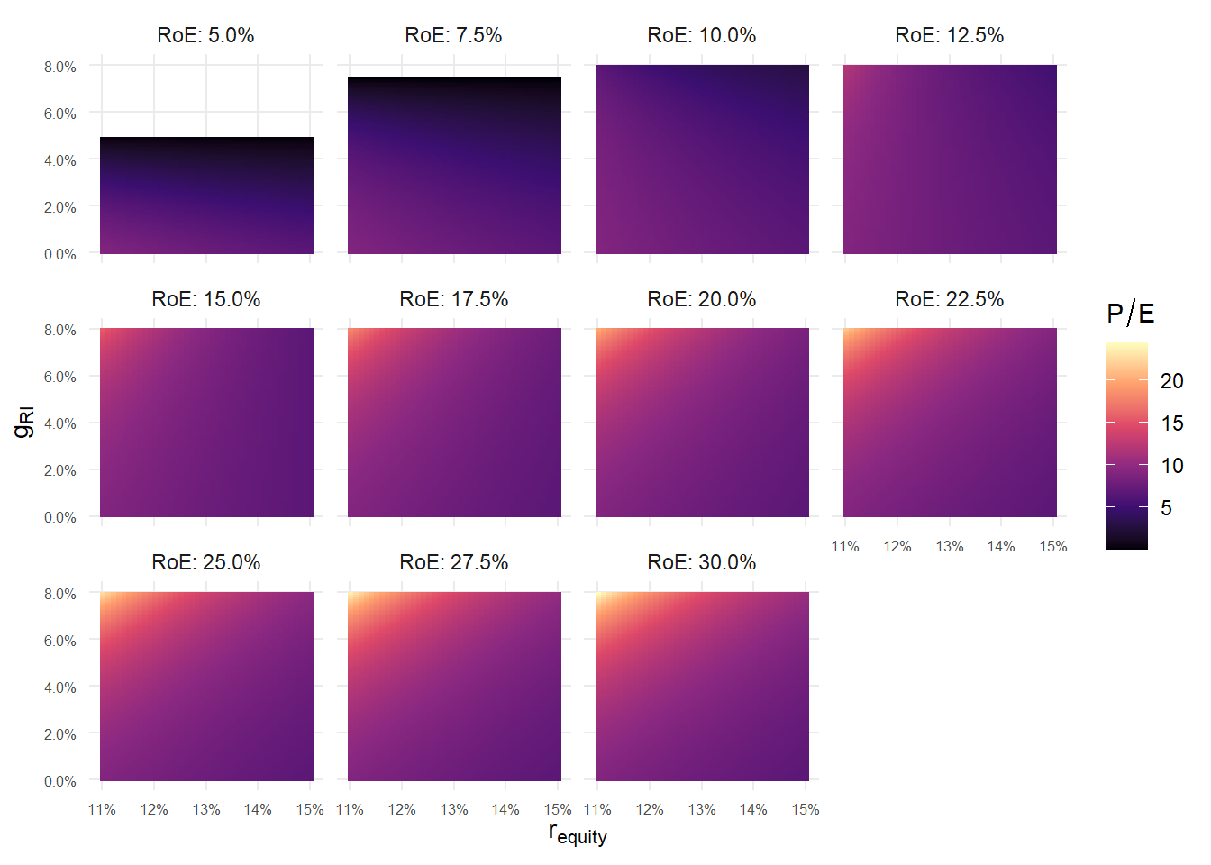
The formula above does not have a very intuitive form though, so let’s plot it for reasonable ranges of \(r_{CE}\), \(g_{RI}\), and \(RoE\)):
library(ggplot2)
library(dplyr)
library(viridisLite)
pe <- function(r, g, RoE){
  (1 / (r - g)) * (1 - (g / RoE))
}

# some reasonable range of value driver values
value_grid <- expand.grid(r   = seq(0.11, 0.15, 0.001),
                          g   = seq(0, 0.08, 0.001),
                          RoE = seq(0.05, 0.3, 0.025)
                          )


pe_data <- as.data.frame(value_grid)
pe_data$PE = pe(pe_data$r, pe_data$g, pe_data$RoE)
pe_data$RoE <- factor(
  paste("RoE:", scales::percent(pe_data$RoE)),
  levels = c("RoE: 5.0%", "RoE: 7.5%", "RoE: 10.0%", "RoE: 12.5%",
             "RoE: 15.0%", "RoE: 17.5%", "RoE: 20.0%", "RoE: 22.5%",
             "RoE: 25.0%", "RoE: 27.5%",  "RoE: 30.0%")
)
pe_plots <-
  pe_data %>%
  filter(
    is.infinite(PE) == FALSE,
    PE > 0
  ) %>%
  ggplot(aes(x = r, y = g, fill = PE)) +
  geom_raster() +
  facet_wrap(~RoE) +
  labs(
    x = expression(r[equity]),
    y = expression(g[RI]),
    fill = expression(P/E)
  ) +
  scale_fill_viridis_c(option = "A") +
  scale_x_continuous(labels = function(x) paste0(round(x*100, 0), "%")) +
  scale_y_continuous(labels=scales::percent) +
  theme_minimal() +
  theme(axis.text = element_text(size = 6),
        panel.grid.minor = element_blank())
pe_plots
And because this picture is not as helpful as could be (and I wanted an excuse to fiddle with the fabulous rayshader package), here is the same plot in 3D:

The main points are:
- Generally P/E is highest for high growth relative to risk (the upper left corner). Profitability has a positive moderating effect. Higher return on equity “bends” the plane further upwards by the upper left corner. The only exception (unsurprisingly) are those facets where RoE < r. In this case residual income–the abnormal profits–are negative. Which means the company is destroying value. Higher growth just means the company is destroying value faster, which is why the PE plane curves down with higher growth for the RoE < r cases.
- Back to the original question: Finding similar firms doesn’t mean just taking firms in the same industry per-se. It means finding firms with similar risk (
\(r\)), growth (\(g\)), and profitability (\(RoE\)) profile. Naturally, firms in the same market will likely have the same market risk, market growth opportunities, etc. So those are good candidates. But you’d still want to think about this further. For example, if two firms compete, they could have different competitive advantages and different profitability characteristics. One firm’s growth could come at the expense of the other. - Note that different combinations, of
\(r\),\(g\),\(RoE\)can give you similar multiples. For example, both combinations, r = 13%, g = 2.5%, and RoE: 25.0% and R = 14%, g = 7%, and RoE: 17.5% lead to a PE of 8.6. But, even though they have the same multiple right now, since they are on different slopes in this valuation space, the multiples will change differently, if things change. This just reiterates that you want to look for comparables with the same\(r\),\(g\),\(RoE\)profile, because only then will changes in multiples be similar, if things change.
Takeaways
Multiple valuation means finding similar firms and applying their valuation–just following the logic that similar assets should be valued similarly. The tricky part is finding similar firms. What this small note hopefully showed is that similar firms are those with similar expected risk, growth, and profitability profiles. Quantifying those in the first place is of course not trivial (and depending on how detailed you do this, you probably do not need to resort to multiples anymore). For example, growth in abnormal profits \(g_{ri}\) is hard to reason about–as compared to, for example, growth in sales. But, even just ballparking whether the business models are comparable in terms of general risk, growth, and profitability prospects will already prevent clearly wrong comparables from entering the valuation.
Full code
library(ggplot2)
library(dplyr)
library(viridisLite)
library(rayshader)
library(rgl)

pe <- function(r, g, RoE){
  (1 / (r - g)) * (1 - (g / RoE))
}

value_grid <- expand.grid(r = seq(0.11, 0.15, 0.001),
                          g = seq(0, 0.08, 0.001),
                          RoE = seq(0.05, 0.3, 0.025)
)


pe_data <- as.data.frame(value_grid)
pe_data$PE = pe(pe_data$r, pe_data$g, pe_data$RoE)
pe_data$RoE <- factor(
  paste("RoE:", scales::percent(pe_data$RoE)),
  levels = c("RoE: 5.0%", "RoE: 7.5%", "RoE: 10.0%", "RoE: 12.5%",
             "RoE: 15.0%", "RoE: 17.5%", "RoE: 20.0%", "RoE: 22.5%",
             "RoE: 25.0%", "RoE: 27.5%",  "RoE: 30.0%")
)


pe_plots <-
  pe_data %>%
  filter(
    is.infinite(PE) == FALSE,
    PE > 0
  ) %>%
  ggplot(aes(x = r, y = g, fill = PE)) +
  geom_raster() +
  facet_wrap(~RoE) +
  labs(
    x = expression(r[equity]),
    y = expression(g[RI]),
    fill = expression(P/E)
  ) +
  scale_fill_viridis_c(option = "A") +
  scale_x_continuous(labels = function(x) paste0(round(x*100, 0), "%")) +
  scale_y_continuous(labels=scales::percent) +
  theme_minimal() +
  theme(axis.text = element_text(size = 6),
        panel.grid.minor = element_blank())
pe_plots


plot_gg(
  pe_plots,
  multicore = TRUE,
  width = 6,
  height = 6,
  scale = 250,
  windowsize = c(1400, 866),
  zoom = 0.45, theta = -40, phi = 30
)

render_movie(
  filename = 'pe',
  type = "orbit",
  phi = 30,
  zoom = 0.45,
  theta = -40
)