library(tidyverse)
library(cmdstanr)
library(posterior)
library(patchwork)
source("00-utils.R")
kable <- knitr::kable
theme_set(theme_prodgray())

ols_erc <- function(.d){
  fit <- lm(ret_dm ~ earn_surp_dm, data = .d)
  fit_results <- broom::tidy(fit)
}

ols_pred <- function(.d){
  fit <- lm(ret_dm ~ earn_surp_dm, data = .d)
  fit_pred <- broom::augment(fit)
}
1. Introduction and preliminaries
This markdown file contains all the code necessary to replicate the main figures, models and results used in Section 3: Heterogeneity in earnings response coefficients of the Paper What Can Bayesian Inference Do for Accounting Research?. The prior predictive checks and the cross-validation test are on separate pages. All the code can also be found in the repo. It contains 00-utils.R which contains a few helper functions for graphs and tables.
Note: I used the newer cmdstanr package instead of the older rstan package because it likely is the future of the R based Stan ecosystem. I also really like its api, which is very close to the api of the pystan package. An additional advantage (I hope) is thus that most model fitting code should be more or less directly transferable to pystan for those that want to work in python. Installing cmdstanr used to be tricky at times because one needs a working c++ toolchain. But it is much smoother now. Please see the cmdstanr doc for installation instructions
2. Loading the data
2.1. Final transformations
The data used here is generated via the 02-create-ERC-sample.R script found in the repo. Here, we just load it and do some last minute transformations like de-meaning, etc.
ea_data <- arrow::read_parquet("../data/ea-event-returns.pqt")
ea_data <-
  ea_data |>
  mutate(
    ret_dm = AbEvRet - mean(AbEvRet),
    earn_surp_dm = earn_surp - mean(earn_surp)
    )
head(ea_data) |>
  kable()
| ticker | permno | fpend_date | ea_date | actual_eps | median_fcast_eps | num_forecasts | two_days_bef_ea | Price | earn_surp | ea_match_date | AbEvRet | firm_id | ret_dm | earn_surp_dm |
|---|---|---|---|---|---|---|---|---|---|---|---|---|---|---|
| 001N | 14504 | 2014-12-31 | 2015-02-09 | 0.04 | 0.030 | 3 | 2015-02-05 | 14.49 | 0.0006901 | 2015-02-09 | -0.2428478 | 1 | -0.2472159 | 0.0006950 |
| 001N | 14504 | 2015-03-31 | 2015-05-05 | 0.06 | -0.045 | 4 | 2015-05-01 | 12.42 | 0.0084541 | 2015-05-05 | -0.0452097 | 1 | -0.0495779 | 0.0084589 |
| 001N | 14504 | 2015-06-30 | 2015-08-05 | 0.02 | -0.015 | 4 | 2015-08-03 | 9.25 | 0.0037838 | 2015-08-05 | 0.0469699 | 1 | 0.0426018 | 0.0037886 |
| 001N | 14504 | 2015-09-30 | 2015-11-04 | -0.02 | 0.040 | 5 | 2015-11-02 | 5.82 | -0.0103093 | 2015-11-04 | 0.0769411 | 1 | 0.0725729 | -0.0103044 |
| 002T | 14503 | 2014-06-30 | 2014-08-07 | 0.19 | 0.235 | 4 | 2014-08-05 | 33.33 | -0.0013501 | 2014-08-07 | -0.0166244 | 2 | -0.0209926 | -0.0013453 |
| 002T | 14503 | 2014-09-30 | 2014-11-04 | 0.18 | 0.340 | 5 | 2014-10-31 | 30.43 | -0.0052580 | 2014-11-04 | -0.0211484 | 2 | -0.0255165 | -0.0052531 |
ea_data_time <-
  ea_data |>
  mutate(EAYear = lubridate::year(ea_date)) |>
  mutate(year_id = as.integer(EAYear - min(EAYear) + 1))
2.2. Tab. 1, Panel A.
desc_tabl <- rbind(
  desc_row(ea_data$AbEvRet, "Ret"),
  desc_row(ea_data$earn_surp, "X")
)
desc_tabl$N <- nrow(ea_data)
desc_tabl$Firms <- max(ea_data$firm_id)

write_csv(desc_tabl, "../out/results/tab1-panA.csv")

desc_tabl|>
  mutate(across(where(is.numeric), round, 4)) |>
  kable()
| var | mean | sd | q5 | q25 | q50 | q75 | q95 | N | Firms | |
|---|---|---|---|---|---|---|---|---|---|---|
| 5% | Ret | 0.0044 | 0.0779 | -0.1252 | -0.0394 | 0.0027 | 0.0470 | 0.1392 | 67360 | 2966 |
| 5%1 | X | 0.0000 | 0.0044 | -0.0075 | -0.0005 | 0.0003 | 0.0014 | 0.0056 | 67360 | 2966 |
3. OLS estimates
3.1 Pooled OLS estimates
Just to have a frame of reference, here is the pooled ERC estimate
pooled <- ols_erc(ea_data)
kable(pooled)
| term | estimate | std.error | statistic | p.value |
|---|---|---|---|---|
| (Intercept) | 0.000000 | 0.0002955 | 0.00000 | 1 |
| earn_surp_dm | 3.116373 | 0.0665200 | 46.84867 | 0 |
3.2 Firm-level OLS estimates
Next, we nest the data by firm (ticker) and fit OLS ERC models by firm
nested_data <-
  ea_data %>%
  add_count(ticker, name = "n_EAs") %>%
  nest(data = -c(ticker, n_EAs, firm_id)) %>%
  mutate(ols_result = map(.x = data, .f = ~ols_erc(.)))

summary(nested_data$n_EAs)
   Min. 1st Qu.  Median    Mean 3rd Qu.    Max.
1.00 4.00 13.00 22.71 33.00 122.00 This is the distribution of firm-level ERC estimates
summary(ols_results$estimate)
     Min.   1st Qu.    Median      Mean   3rd Qu.      Max.      NA's
-5034.136     0.068     3.884     6.041    10.650  5462.750       294
3.3 By-year OLS estimates
This is for the comparison in Figure 5.
byyear_data <-
  ea_data_time %>%
  nest(data = -c(year_id, EAYear)) %>%
  mutate(ols_result = map(.x = data, .f = ~ols_erc(.)))
byyear_results <-
  byyear_data %>%
  select(-data) %>%
  unnest(ols_result) %>%
  filter(term == "earn_surp_dm")
4. Bayesian model with weakly informative priors
4.1 Model fitting
To fit a Bayesian model I use Stan, or, more precisely, its R bindings in cmdstanr. To fit a Bayesian model, we need to:
- Write the corresponding model using the Stan language
- Compile the code into a Stan model executable (an .exe file)
- Make a list of data to feed into the .exe file
- Let the model run and generate MCMC chains (or whatever algorithm is specified)
The model itself is coded in the Stan language. There are many excellent tutorials on Stan available online. So I won’t waste space explaining it here. For various reasons (e.g., debugging) it is customary to put the model code in a separate .stan file. All the model files can be found in the /Stan/ folder of the repo.
cat(read_lines("../Stan/erc-wkinfo-priors.stan"), sep = "\n")
data{
  int<lower=1> N;                   // num obs
  int<lower=1> J;                   // num groups
  int<lower=1> K;                   // num coefficients
  int<lower=1, upper=J> GroupID[N]; // GroupID for obs, e.g. FirmID or Industry-YearID
  vector[N] y;                      // Response
  matrix[N, K] x;                   // Predictors (incl. Intercept)
}
parameters{
  matrix[K, J] z;                  // standard normal sampler
  cholesky_factor_corr[K] L_Omega; // hypprior coefficient correlation
  vector<lower=0>[K] tau;          // hypprior coefficient scales
  vector[K] mu_b;                  // hypprior mean coefficients
  real<lower=0> sigma;             // error-term scale
}
transformed parameters{
  matrix[J, K] b;                  // coefficient vector
  // The multivariate non-centered version:
  b = (rep_matrix(mu_b, J) + diag_pre_multiply(tau,L_Omega) * z)';
}
model{
  to_vector(z) ~ normal(0, 1);
  L_Omega ~ lkj_corr_cholesky(2);
  mu_b[1]  ~ normal(0, 0.1);
  mu_b[2]  ~ normal(0, 40);
  sigma ~ exponential(1.0 / 0.08);   // exp: 0.08 (std (abnormal returns))
  tau[1] ~ exponential(1.0 / 0.1);   // exp: 0.1
  tau[2] ~ exponential(1.0 / 40);    // exp: 40
  y ~ normal(rows_dot_product(b[GroupID] , x), sigma);
}
// generated quantities {
//   array[N] real y_pred = normal_rng(rows_dot_product(b[GroupID] , x), sigma);
// }Next, we compile the model to an .exe file
model_wkinfo_priors <- cmdstan_model("../Stan/erc-wkinfo-priors.stan")
Now, we prepare the list of data to feed into the model.
input_data <- list(
  N = nrow(ea_data),
  J = max(ea_data$firm_id),
  K = 2,
  GroupID = ea_data$firm_id,
  y = ea_data$AbEvRet,
  x = as.matrix(data.frame(int = 1, esurp = ea_data$earn_surp))
)
We run the model
Beware, this fit can take a long time
fit_wkinfo_priors <- model_wkinfo_priors$sample(
  data = input_data,
  iter_sampling = 1000,
  iter_warmup = 1000,
  chains = 4,
  parallel_chains = 4,
  seed = 1234,
  refresh = 1000
)
Running MCMC with 4 parallel chains...

Chain 1 Iteration:    1 / 2000 [  0%]  (Warmup)
Chain 2 Iteration:    1 / 2000 [  0%]  (Warmup)
Chain 3 Iteration:    1 / 2000 [  0%]  (Warmup)
Chain 4 Iteration:    1 / 2000 [  0%]  (Warmup)
Chain 1 Iteration: 1000 / 2000 [ 50%]  (Warmup)
Chain 1 Iteration: 1001 / 2000 [ 50%]  (Sampling)
Chain 4 Iteration: 1000 / 2000 [ 50%]  (Warmup)
Chain 4 Iteration: 1001 / 2000 [ 50%]  (Sampling)
Chain 2 Iteration: 1000 / 2000 [ 50%]  (Warmup)
Chain 2 Iteration: 1001 / 2000 [ 50%]  (Sampling)
Chain 3 Iteration: 1000 / 2000 [ 50%]  (Warmup)
Chain 3 Iteration: 1001 / 2000 [ 50%]  (Sampling)
Chain 3 Iteration: 2000 / 2000 [100%]  (Sampling)
Chain 3 finished in 1941.6 seconds.
Chain 4 Iteration: 2000 / 2000 [100%]  (Sampling)
Chain 4 finished in 1962.7 seconds.
Chain 1 Iteration: 2000 / 2000 [100%]  (Sampling)
Chain 1 finished in 2088.8 seconds.
Chain 2 Iteration: 2000 / 2000 [100%]  (Sampling)
Chain 2 finished in 2132.0 seconds.

All 4 chains finished successfully.
Mean chain execution time: 2031.3 seconds.
Total execution time: 2132.6 seconds.
4.2 Summary of the posterior for selected parameters
Here is the summary of the resulting posterior distribution of the model parameters
fit_wkinfo_priors$summary(variables = c("mu_b", "sigma", "tau", "L_Omega[2,1]")) |>
  mutate(across(where(is.numeric), round, 3)) |>
  kable()
| variable | mean | median | sd | mad | q5 | q95 | rhat | ess_bulk | ess_tail |
|---|---|---|---|---|---|---|---|---|---|
| mu_b[1] | 0.004 | 0.004 | 0.000 | 0.000 | 0.003 | 0.004 | 1.000 | 3943.605 | 3333.804 |
| mu_b[2] | 3.669 | 3.668 | 0.107 | 0.108 | 3.490 | 3.850 | 1.001 | 2575.785 | 2404.202 |
| sigma | 0.076 | 0.076 | 0.000 | 0.000 | 0.075 | 0.076 | 1.003 | 4585.697 | 2582.434 |
| tau[1] | 0.006 | 0.006 | 0.001 | 0.001 | 0.005 | 0.007 | 1.000 | 1037.872 | 2015.912 |
| tau[2] | 2.804 | 2.802 | 0.125 | 0.125 | 2.600 | 3.008 | 1.002 | 1347.643 | 2243.416 |
| L_Omega[2,1] | -0.020 | -0.024 | 0.088 | 0.086 | -0.161 | 0.130 | 1.011 | 276.749 | 683.598 |
4.3 Comparing Bayesian ERC estimates to OLS estimates
To do this we need to extract the posterior draws for the ERC coefficients
posterior_b <- summarise_draws(fit_wkinfo_priors$draws(c("b")),
                               posterior_mean = mean,
                               posterior_sd = sd,
                               ~quantile2(., probs = c(0.05, 0.25, 0.75, 0.95))
                               )
write_csv(posterior_b, "../out/results/fit_wkinfo_bi.csv")

posterior_erc <-
  posterior_b |>
  filter(str_detect(variable, ",2\\]"))
Code for Tab. 1, Panel C
tab1.C <-
  rbind(
    desc_row(posterior_erc$posterior_mean, "post_mean"),
    desc_row(with(posterior_erc, q95 - q5), "post90_width"),
    desc_row(with(ols_results, estimate[is.na(estimate) == FALSE]), "OLS"),
    desc_row(with(ols_results, p.value[is.na(p.value) == FALSE]), "OLS pval")
  )
write_csv(tab1.C, "../out/results/tab1-panC.csv")
tab1.C |>
  mutate(across(where(is.numeric), round, 3))
             var  mean      sd      q5   q25   q50    q75    q95
5%     post_mean 3.672   1.414   1.292 2.970 3.676  4.288  6.105
5%1 post90_width 7.837   1.440   4.946 6.933 8.314  9.013  9.345
5%2          OLS 6.041 178.593 -18.689 0.068 3.884 10.650 45.904
5%3     OLS pval 0.362   0.309   0.002 0.068 0.301  0.611  0.927
4.4 Figure 4
graph_data <-
  ols_results %>%
  mutate(
    post_mean = posterior_erc$posterior_mean,
    post_sd = posterior_erc$posterior_sd
  )
y_range <- c(-100, 100)

f4.panA <-
  graph_data %>%
  ggplot(aes(x = n_EAs, y = estimate)) +
  geom_point(alpha = 0.1, size = 1) + # ,  width = 0.25) +
  geom_hline(yintercept = c(0)) +
  geom_hline(yintercept = mean(graph_data$estimate, na.rm = TRUE), linetype = "dashed") +
  labs(
    y = "OLS estimate",
    x = NULL, # "Nr of Quarters in firm's time series",
    subtitle = "OLS by firm"
  ) +
  coord_cartesian(ylim = y_range)

f4.panB <-
  graph_data %>%
  ggplot(aes(x = n_EAs, y = post_mean)) +
  geom_point(alpha = 0.1, size = 1) + # ,  width = 0.25) +
  geom_hline(yintercept = c(0)) +
  geom_hline(yintercept = mean(graph_data$post_mean), linetype = "dashed") +
  labs(
    y = "Posterior mean",
    x = NULL,
    subtitle = "Bayesian multi-level model"
  ) +
  coord_cartesian(ylim = y_range)


f4.panC <-
  graph_data %>%
  ggplot(aes(x = n_EAs)) +
  geom_bar(width = 0.5) +
  scale_y_continuous(expand = expansion(mult = c(0, 0.05))) +
  labs(
    x = "Time series length",
    y = "N. firms"
  )

fig4 <-
  f4.panA + f4.panB + f4.panC + f4.panC +
  plot_layout(ncol = 2, heights = c(2, 0.5)) +
  plot_annotation(tag_levels = list(c("A", "B", NULL, NULL))) &
  theme(legend.position = "none")
fig4
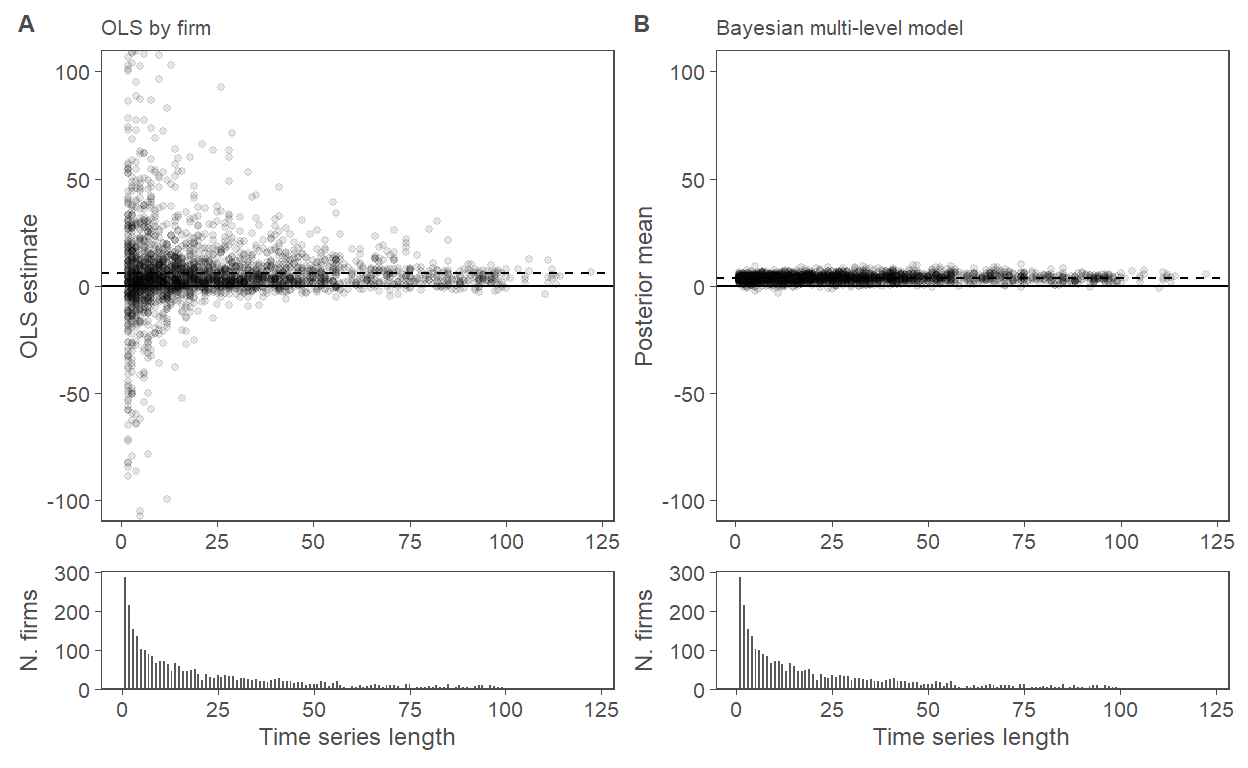
Saving figure
save_fig(fig4, figname = "fig4", w = 6.2, h = 3.4)
5. Bayesian model with AR1 time trend
5.1 Model fitting
cat(read_lines("../Stan/erc-wkinfo-priors-time-pers.stan"), sep = "\n")
data{
  int<lower=1> N;                   // num obs
  int<lower=1> J;                   // num groups
  int<lower=1> K;                   // num coefficients
  int<lower=1> M;                   // num periods
  int<lower=1, upper=J> GroupID[N]; // GroupID for obs, e.g. FirmID or Industry-YearID
  int<lower=1, upper=M> TimeID[N];  // GroupID for obs, e.g. FirmID or Industry-YearID
  vector[N] y;                      // Response
  vector[N] x;                      // Predictor (without Intercept)
}
parameters{
  matrix[K, J] z;                  // standard normal sampler
  cholesky_factor_corr[K] L_Omega; // hypprior coefficient correlation
  vector<lower=0>[K] tau;          // hypprior coefficient scales
  real<lower=0> sigma;             // error-term scale
  real mu_0;

  real<lower=0,upper=1> rho_raw;   // used to construct rho, the AR(1) coefficient
  real<lower=0> sig_t;             // error-term scale
  vector[M] z_t;
}
transformed parameters{
  matrix[J, K] b_i;                // firm-level components
  vector[K] mu_b;                  // hypprior mean firm-level coefficients
  // The multivariate non-centered version:
  mu_b[1] = mu_0;
  mu_b[2] = 0;
  b_i = (rep_matrix(mu_b, J) + diag_pre_multiply(tau,L_Omega) * z)';

  // non-centered parameterization of AR(1) process priors
  real rho = 2 * rho_raw - 1;      // ensures that rho is between -1 and 1
  vector[M] b_t = sig_t * z_t;     // all of them share this term
  b_t[1] /= sqrt(1 - rho^2);       // mo[1] = mo[1] / sqrt(1 - rho^2)
  for (m in 2:M) {
    b_t[m] += rho * b_t[m-1];      // mo[m] = mo[m] + rho * mo[m-1];
  }

}
model{
  to_vector(z) ~ normal(0, 1);
  z_t ~ normal(0, 1);
  L_Omega ~ lkj_corr_cholesky(2);
  mu_0  ~ normal(0, 0.1);
  rho_raw  ~ beta(10, 5);

  sigma ~ exponential(1.0 / 0.08);   // exp: 0.08 (std (abnormal returns))
  tau[1] ~ exponential(1.0 / 0.1);   // exp: 0.1
  tau[2] ~ exponential(1.0 / 40);    // exp: 40
  sig_t ~ exponential(1.0 / 40);     // exp: 40

  vector[N] n_loc = b_i[GroupID, 1] + (b_t[TimeID] + b_i[GroupID, 2]) .* x;

  y ~ normal(n_loc, sigma);
}model_wkinfo_timepers <- cmdstan_model("../Stan/erc-wkinfo-priors-time-pers.stan")
Again beware, this fit can take a long time
fit_wkinfo_timepers <- model_wkinfo_timepers$sample(
  data = input_data2,
  iter_sampling = 1000,
  iter_warmup = 1000,
  chains = 4,
  parallel_chains = 4,
  seed = 1234,
  refresh = 1000
)
Running MCMC with 4 parallel chains...

Chain 2 Iteration:    1 / 2000 [  0%]  (Warmup)
Chain 4 Iteration:    1 / 2000 [  0%]  (Warmup)
Chain 1 Iteration:    1 / 2000 [  0%]  (Warmup)
Chain 3 Iteration:    1 / 2000 [  0%]  (Warmup)
Chain 3 Iteration: 1000 / 2000 [ 50%]  (Warmup)
Chain 3 Iteration: 1001 / 2000 [ 50%]  (Sampling)
Chain 2 Iteration: 1000 / 2000 [ 50%]  (Warmup)
Chain 2 Iteration: 1001 / 2000 [ 50%]  (Sampling)
Chain 1 Iteration: 1000 / 2000 [ 50%]  (Warmup)
Chain 1 Iteration: 1001 / 2000 [ 50%]  (Sampling)
Chain 4 Iteration: 1000 / 2000 [ 50%]  (Warmup)
Chain 4 Iteration: 1001 / 2000 [ 50%]  (Sampling)
Chain 3 Iteration: 2000 / 2000 [100%]  (Sampling)
Chain 3 finished in 2301.3 seconds.
Chain 1 Iteration: 2000 / 2000 [100%]  (Sampling)
Chain 1 finished in 2386.3 seconds.
Chain 2 Iteration: 2000 / 2000 [100%]  (Sampling)
Chain 2 finished in 2400.0 seconds.
Chain 4 Iteration: 2000 / 2000 [100%]  (Sampling)
Chain 4 finished in 2537.5 seconds.

All 4 chains finished successfully.
Mean chain execution time: 2406.3 seconds.
Total execution time: 2538.0 seconds.
5.2 Summary of the posterior for selected parameters
Here is the summary of the resulting posterior distribution of the model parameters
fit_wkinfo_timepers$summary(variables = c("mu_b[1]", "sigma", "tau", "b_t",
                                          "rho", "sig_t", "L_Omega[2,1]")) |>
  mutate(across(where(is.numeric), round, 3)) |>
  kable()
| variable | mean | median | sd | mad | q5 | q95 | rhat | ess_bulk | ess_tail |
|---|---|---|---|---|---|---|---|---|---|
| mu_b[1] | 0.003 | 0.003 | 0.000 | 0.000 | 0.003 | 0.004 | 1.004 | 4608.601 | 3102.494 |
| sigma | 0.075 | 0.075 | 0.000 | 0.000 | 0.075 | 0.076 | 1.000 | 3703.130 | 2184.654 |
| tau[1] | 0.006 | 0.006 | 0.001 | 0.001 | 0.005 | 0.007 | 1.001 | 1072.303 | 1881.667 |
| tau[2] | 2.615 | 2.612 | 0.122 | 0.118 | 2.419 | 2.821 | 1.005 | 1547.561 | 2254.383 |
| b_t[1] | 1.798 | 1.794 | 0.335 | 0.335 | 1.254 | 2.349 | 1.000 | 6564.086 | 3714.573 |
| b_t[2] | 1.699 | 1.701 | 0.310 | 0.319 | 1.183 | 2.198 | 1.000 | 5728.963 | 3821.598 |
| b_t[3] | 1.967 | 1.971 | 0.299 | 0.298 | 1.491 | 2.462 | 1.000 | 6325.139 | 3566.423 |
| b_t[4] | 2.302 | 2.300 | 0.319 | 0.318 | 1.783 | 2.843 | 1.001 | 5648.104 | 3809.811 |
| b_t[5] | 2.479 | 2.488 | 0.353 | 0.344 | 1.891 | 3.061 | 1.001 | 6555.830 | 3578.803 |
| b_t[6] | 1.969 | 1.971 | 0.326 | 0.333 | 1.424 | 2.495 | 1.000 | 5906.941 | 3710.413 |
| b_t[7] | 2.581 | 2.577 | 0.341 | 0.330 | 2.021 | 3.159 | 1.000 | 5834.040 | 3507.401 |
| b_t[8] | 3.065 | 3.070 | 0.351 | 0.356 | 2.490 | 3.641 | 1.001 | 5946.883 | 3773.475 |
| b_t[9] | 3.043 | 3.039 | 0.346 | 0.336 | 2.482 | 3.622 | 1.000 | 6807.729 | 2933.874 |
| b_t[10] | 2.824 | 2.826 | 0.348 | 0.348 | 2.242 | 3.382 | 1.000 | 6918.646 | 3719.018 |
| b_t[11] | 3.135 | 3.140 | 0.384 | 0.381 | 2.503 | 3.762 | 1.000 | 7432.118 | 3579.078 |
| b_t[12] | 3.175 | 3.176 | 0.383 | 0.392 | 2.540 | 3.799 | 1.001 | 6264.057 | 3811.178 |
| b_t[13] | 3.523 | 3.525 | 0.368 | 0.370 | 2.914 | 4.133 | 0.999 | 6556.955 | 3728.211 |
| b_t[14] | 3.838 | 3.837 | 0.398 | 0.398 | 3.180 | 4.476 | 0.999 | 6121.546 | 3726.720 |
| b_t[15] | 4.461 | 4.459 | 0.409 | 0.406 | 3.788 | 5.148 | 1.000 | 6665.553 | 3867.688 |
| b_t[16] | 5.957 | 5.956 | 0.403 | 0.402 | 5.299 | 6.633 | 1.000 | 5896.254 | 3454.660 |
| b_t[17] | 5.868 | 5.873 | 0.382 | 0.391 | 5.255 | 6.487 | 1.000 | 5911.323 | 3872.781 |
| b_t[18] | 6.461 | 6.453 | 0.394 | 0.397 | 5.827 | 7.104 | 1.001 | 5171.089 | 3228.712 |
| b_t[19] | 4.977 | 4.976 | 0.311 | 0.312 | 4.472 | 5.495 | 1.000 | 5879.135 | 3677.540 |
| b_t[20] | 4.169 | 4.168 | 0.265 | 0.265 | 3.724 | 4.605 | 1.000 | 5316.392 | 3666.933 |
| b_t[21] | 4.704 | 4.693 | 0.310 | 0.307 | 4.197 | 5.218 | 1.002 | 6076.813 | 3584.917 |
| b_t[22] | 5.870 | 5.866 | 0.358 | 0.362 | 5.289 | 6.451 | 1.000 | 5298.588 | 3418.853 |
| b_t[23] | 5.561 | 5.566 | 0.389 | 0.392 | 4.917 | 6.199 | 1.002 | 6182.931 | 3860.695 |
| b_t[24] | 4.562 | 4.567 | 0.441 | 0.446 | 3.835 | 5.281 | 1.000 | 5299.736 | 3824.800 |
| b_t[25] | 5.096 | 5.094 | 0.442 | 0.442 | 4.377 | 5.835 | 1.001 | 5638.985 | 3851.835 |
| b_t[26] | 5.659 | 5.664 | 0.444 | 0.446 | 4.944 | 6.378 | 1.000 | 7011.250 | 3646.906 |
| b_t[27] | 5.719 | 5.716 | 0.488 | 0.479 | 4.920 | 6.516 | 1.002 | 6129.497 | 3780.013 |
| b_t[28] | 6.448 | 6.438 | 0.612 | 0.603 | 5.446 | 7.467 | 1.001 | 6038.999 | 3444.120 |
| b_t[29] | 5.667 | 5.654 | 0.604 | 0.610 | 4.678 | 6.646 | 1.001 | 5950.123 | 3377.044 |
| b_t[30] | 4.365 | 4.346 | 0.601 | 0.607 | 3.415 | 5.365 | 1.000 | 5965.089 | 3543.557 |
| b_t[31] | 1.624 | 1.622 | 0.600 | 0.591 | 0.644 | 2.604 | 1.000 | 4175.004 | 3838.545 |
| rho | 0.894 | 0.898 | 0.037 | 0.035 | 0.828 | 0.948 | 1.000 | 2739.444 | 2701.058 |
| sig_t | 1.077 | 1.057 | 0.196 | 0.185 | 0.794 | 1.430 | 1.001 | 1669.068 | 2703.365 |
| L_Omega[2,1] | 0.133 | 0.131 | 0.093 | 0.091 | -0.021 | 0.292 | 1.007 | 382.611 | 631.552 |
Saving output for Panel E of Tab. 1
5.3 Comparing Bayesian ERC estimates to OLS estimates
posterior_b2 <- summarise_draws(fit_wkinfo_timepers$draws(c("b_i")),
                               posterior_mean = mean,
                               posterior_sd = sd,
                               ~quantile2(., probs = c(0.05, 0.25, 0.75, 0.95))
                               )
posterior_erc2 <-
  posterior_b2 |>
  filter(str_detect(variable, ",2\\]"))

posterior_bt2 <- summarise_draws(fit_wkinfo_timepers$draws(c("b_t")),
                                 posterior_mean = mean,
                                 posterior_sd = sd,
                                 ~quantile2(., probs = c(0.05, 0.25, 0.75, 0.95))
                                 )

write_csv(posterior_bt2, "../out/results/fit_wkinfo_time_bt.csv")
write_csv(posterior_b2, "../out/results/fit_wkinfo_time_bi.csv")
fit_comparison2 <-
  rbind(
    desc_row(posterior_erc2$posterior_mean, "post_mean"),
    desc_row(with(posterior_erc2, q95 - q5), "post90_width"),
    desc_row(with(ols_results, estimate[is.na(estimate) == FALSE]), "OLS")
  )
write_csv(fit_comparison2, "../out/results/fit_comp-AR1.csv")

fit_comparison2 |>
  mutate(across(where(is.numeric), round, 3)) |>
  kable()
| var | mean | sd | q5 | q25 | q50 | q75 | q95 | |
|---|---|---|---|---|---|---|---|---|
| 5% | post_mean | 0.004 | 1.273 | -2.213 | -0.548 | 0.007 | 0.598 | 2.153 |
| 5%1 | post90_width | 7.410 | 1.259 | 4.847 | 6.664 | 7.835 | 8.413 | 8.733 |
| 5%2 | OLS | 6.041 | 178.593 | -18.689 | 0.068 | 3.884 | 10.650 | 45.904 |
Compare this to the numbers from the model without time trend
tab1.C |>
  mutate(across(where(is.numeric), round, 3)) |>
  kable()
| var | mean | sd | q5 | q25 | q50 | q75 | q95 | |
|---|---|---|---|---|---|---|---|---|
| 5% | post_mean | 3.672 | 1.414 | 1.292 | 2.970 | 3.676 | 4.288 | 6.105 |
| 5%1 | post90_width | 7.837 | 1.440 | 4.946 | 6.933 | 8.314 | 9.013 | 9.345 |
| 5%2 | OLS | 6.041 | 178.593 | -18.689 | 0.068 | 3.884 | 10.650 | 45.904 |
| 5%3 | OLS pval | 0.362 | 0.309 | 0.002 | 0.068 | 0.301 | 0.611 | 0.927 |
5.4 Fig. 5
posterior_bt2 |>
  mutate(Year = 1:nrow(posterior_bt2) + 1989) |>
  left_join(select(byyear_results, Year = EAYear, OLS = estimate),
            by = c("Year")) |>
  ggplot(aes(x = Year)) +
  geom_ribbon(aes(ymin = q5, ymax = q95), alpha = 0.2) +
  geom_ribbon(aes(ymin = q25, ymax = q75), alpha = 0.2) +
  geom_line(aes(y = posterior_mean)) +
  geom_line(aes(y = OLS), linetype = 2) +
  scale_x_continuous(breaks = seq(1990, 2020, 5)) +
  scale_y_continuous(limits = c(0, 8), expand = expansion(mult = c(0, 0))) +
  labs(subtitle = expression("Yearly trend component"~a1[t]~"in ERCs"),
       y = "Mean, 50%, and 90% interval",
       x = "Calendar year of the announcement")
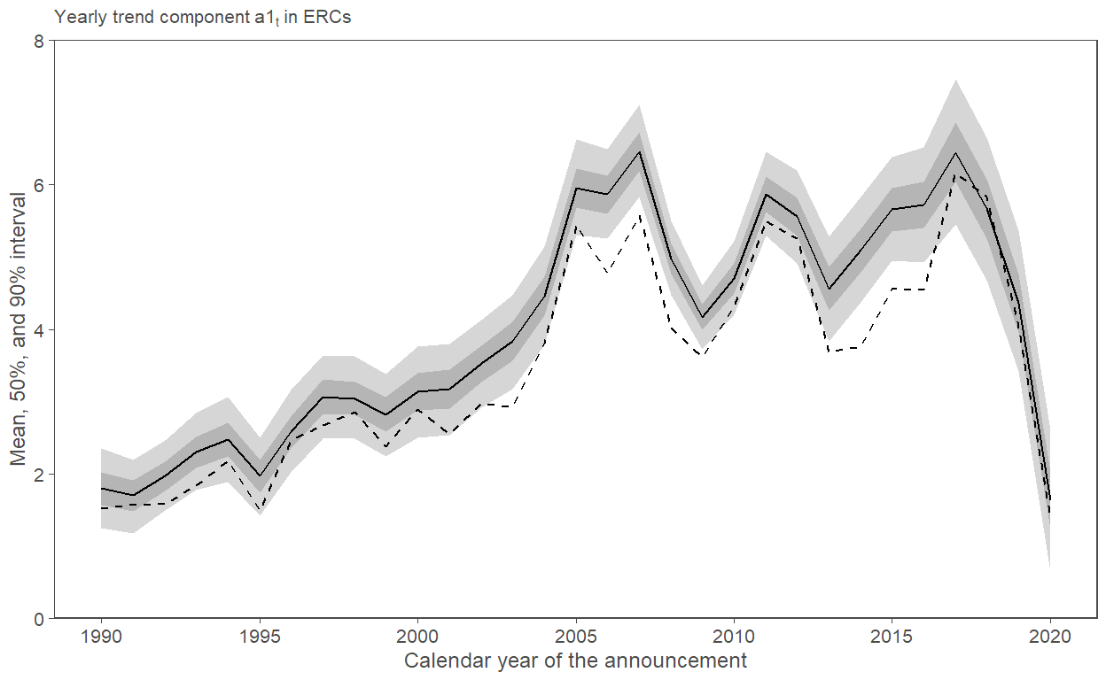
f5.panA <-
  posterior_bt2 |>
  mutate(Year = 1:nrow(posterior_bt2) + 1989) |>
  left_join(select(byyear_results, Year = EAYear, OLS = estimate),
            by = c("Year")) |>
  ggplot(aes(x = Year)) +
  geom_ribbon(aes(ymin = q5, ymax = q95), alpha = 0.2) +
  geom_ribbon(aes(ymin = q25, ymax = q75), alpha = 0.2) +
  geom_line(aes(y = posterior_mean)) +
  geom_line(aes(y = OLS), linetype = 2, color = "grey40") +
  scale_x_continuous(breaks = seq(1990, 2020, 5)) +
  scale_y_continuous(limits = c(0, 8), expand = expansion(mult = c(0, 0))) +
  labs(subtitle = expression("Yearly trend component"~a[1*","*t]~"in ERCs"),
       y = "Mean, 50%, and 90% interval",
       x = "Calendar year of the announcement") +
  annotate("text", label = "OLS estimates", x = 2015.5, y = 3.3, size = 3, color = "grey40") +
  annotate("text", label = "Bayes posterior", x = 2004, y = 7.5, size = 3)

f5.panB <-
  posterior_erc2 |>
  mutate(rank = rank(posterior_mean)) |>
  ggplot(aes(x = rank, y = posterior_mean)) +
  geom_hline(yintercept = 0) +
  geom_linerange(aes(ymin = q5, ymax = q95), alpha = 0.1) +
  geom_point(size = 0.5) +
  scale_x_continuous(expand = expansion(mult = c(0.01, 0.01))) +
  labs(y = "Mean and 90% interval",
       x = expression(a[1*","*i]~"rank"),
       subtitle = expression("Firm-individual ERC component"~a[1*","*i]~"from smallest to largest"))

fig5 <-
  f5.panA / f5.panB +
  plot_annotation(tag_levels = "A") &
  theme(legend.position = "none")
fig5
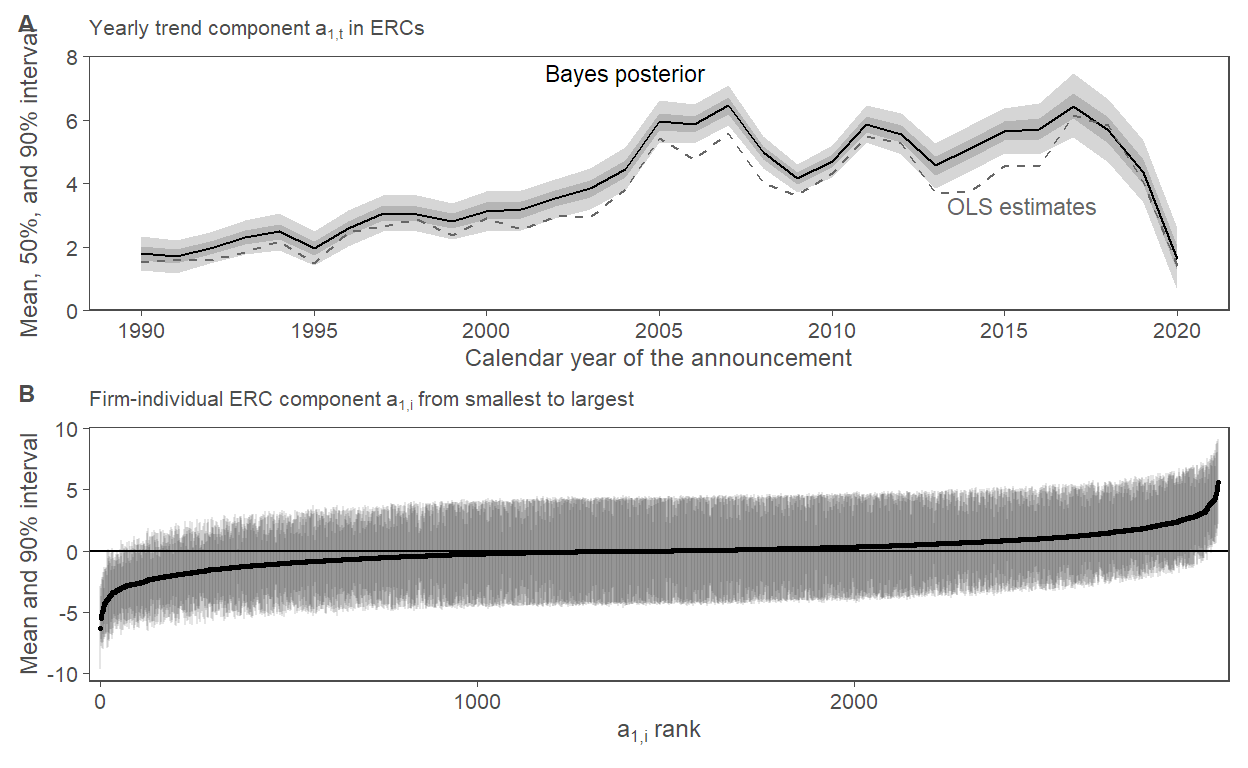
Saving figure
save_fig(fig5, figname = "fig5", w = 6.2, h = 5)