1. Introduction
Consider the simulation in Section 2, of the paper:
\[y = a_0 + a_1 * x + \epsilon, \, \epsilon \sim N(0, \sigma)\] \[a_0 \sim N(0, 100)\] \[a_1 \sim N(0, 4)\] \[\sigma \sim Exponential(1/21)\] This note explains the basics of how this model is fit to the simulated data and how draws from the posterior distribution are generated.
Show code
set.seed(888)
n_samples <- 50
n_obs <- 50
x_fix <- rnorm(n = n_obs, 0, 1)
gen_data <- function(n) tibble(u = rnorm(n, 0, 20), x = x_fix, y = 1 + 2 * x_fix + u)

# gen samples
samples <- tibble(id = 1:n_samples)
samples$data <- map(rep.int(n_obs, n_samples), gen_data)
sample1 <- samples$data[[1]]
input_data <- list(
  y = sample1$y,
  x = sample1$x,
  N = nrow(sample1)
)
Show code
model_weak_priors <- cmdstan_model("../Stan/sim-wkinfo-priors.stan")
fit_weak_priors <- model_weak_priors$sample(
  data = input_data,
  iter_sampling = 1000,
  iter_warmup = 1000,
  chains = 4,
  parallel_chains = 4,
  seed = 1234,
  save_warmup = TRUE,
  refresh = 0
)
Running MCMC with 4 parallel chains...

Chain 1 finished in 0.1 seconds.
Chain 3 finished in 0.1 seconds.
Chain 4 finished in 0.1 seconds.
Chain 2 finished in 0.1 seconds.

All 4 chains finished successfully.
Mean chain execution time: 0.1 seconds.
Total execution time: 0.4 seconds.
2. Markov Chain Monte Carlo Sampling
The flexibility gained from working with probability distribution comes at the cost of computational complexity. Even moderately complex models have no analytically tractable posterior distribution. Instead, we use simulation methods to sample from the unknown posterior distribution. These methods, called Markov Chain Monte Carlo methods, draw “chains” of random samples from the unknown posterior (in our example, each sample draw is a triplet (\(a_0\),\(a_1\),\(\sigma\))). A Markov chain is a sequence of random variables \(\theta_1\), \(\theta_2\), … (again, in our example, the triplet (\(a_0\),\(a_1\),\(\sigma\))\(_1\), (\(a_0\),\(a_1\),\(\sigma\))\(_2\),…) where the distribution of \(\theta_t\) depends only on the most recent value \(\theta_{t-1}\). MCMC algorithms do two things: 1) they draw samples of parameter values from an approximation to the unknown posterior and 2) with each draw, the approximation to the actual posterior distribution is improved. Once the chains run long enough to converge to the unknown posterior, the chains will draw (\(a_0\),\(a_1\),\(\sigma\)) in proportion to the unknown posterior probability density of these values.
Show code
postdraws <- fit_weak_priors$draws(format = "draws_df", inc_warmup = TRUE)

graph_data <- as.data.frame(postdraws) |>
  select(-lp__) |>
  filter(.iteration < 1080) |>
  pivot_longer(c(a0, a1, sigma), names_to = "pars")
Show code
graph_data |>
  mutate(pars2 = case_when(
    pars == "a0" ~ "a[0]",
    pars == "a1" ~ "a[1]",
    pars == "sigma" ~ "sigma"
  )) |>
  ggplot(aes(x = .iteration, y = value, group = .chain, color = factor(.chain))) +
  geom_line(alpha = 0.8, size = 0.5) +
  facet_wrap(~pars2, ncol = 1, scales = "free_y", labeller = label_parsed) +
  scale_x_continuous(expand = expansion(mult = c(0.02, 0))) +
  scale_color_grey() +
  labs(
    x = "Iteration",
    y = NULL
    ) +
  theme(legend.position = "bottom")
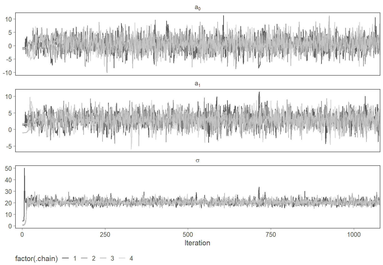
Figure 1: Warmup phase of four MCMC chains
The figure above shows the warmup phase (the first 1,000 iterations) of four Markov chains used to fit the model. Here the convergence happens almost immediately, and the chains traverse the same 3-dimensional space quickly. More likely values will be drawn more often, and less likely values less often. Thus, if the chains are run long enough, we will have empirical samples of the posterior. We can then compute anything we want to know about the posterior (mean, standard deviation, quantiles, etc.) basically by using the histogram of the samples (after discarding the convergence phase, shown below).
Show code
plot_range <- range(range(postdraws$a0), range(postdraws$a0))

fig2.A <-
  postdraws |>
  filter(.iteration > 1000) |>
  ggplot(aes(x = a0)) +
  geom_histogram(binwidth = 0.3) +
  labs(
    x = expression(a[0]),
    y = expression("Number of samples")
  ) +
  scale_x_continuous(expand = c(0, 0), limits = plot_range) +
  scale_y_continuous(expand = expansion(mult = c(0.0, 0.05)))

fig2.B <-
  postdraws |>
  filter(.iteration > 1000) |>
  ggplot(aes(x = a1)) +
  geom_histogram(binwidth = 0.3) +
  labs(
    x = expression(a[1]),
    y = expression("Number of samples")
  ) +
  scale_x_continuous(expand = c(0, 0), limits = plot_range) +
  scale_y_continuous(expand = expansion(mult = c(0.0, 0.05)))

fig2.A / fig2.B
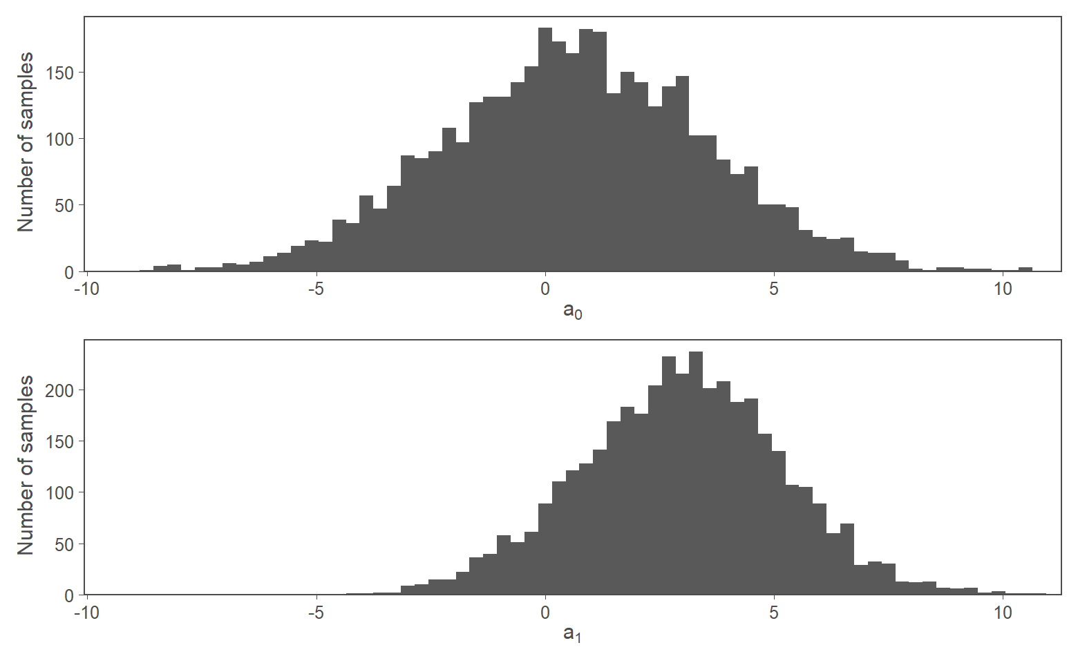
Figure 2: 4,000 MCMC samples from posterior
These histograms are used to reason about the posterior.
There are various algorithms for Markov chains (e.g., Metropolis-Hastings, Gibbs, Hamiltonian Monte Carlo), and developing new ones is an ongoing area of research. A detailed explanation of these algorithms is beyond the scope of this article, and interested readers are referred to Gelman et al. (2014). Here, I will instead focus on what is involved in fitting a Bayesian model using MCMC sampling.
3. Working with Markov Chains
Important choices include how many chains to run in parallel and for how long. It is nearly always advisable to run several chains at once. The length of each chain (the number of iterations of draws) determines whether the chain has enough steps to converge to and then traverse the full posterior. A common starting point for modern MCMC algorithms is to run 4 chains with 2,000 iterations each, discarding the first 1,000 iterations of each chain. The remaining 4,000 iterations from all four chains serve as the empirical samples from the posterior from which we can compute posterior mean, standard deviation, and so on. Running several chains is done for three reasons.
First, for a given set of iterations per chain, the more chains we run, the more samples we have, and thus the more detail about the empirical distribution is available to us. Aspects such as the tails of the posterior (e.g., the 1st or 99th percentile) are only precisely captured if we have many samples (i.e., 1,000+ effective samples).
Alternatively, one could run one very long chain to have many samples. The second reason for running multiple chains, instead of one long chain, is that it helps assess when the chains have converged to the posterior. Markov chains need some iterations to converge to the posterior and start tracing it. This is often called “warm-up” or “burn-in” period and needs to be discarded before drawing any inferences from the samples. A common problem is to assess when such convergence has happened. With only one chain, one can only examine whether the chain is behaving erratically. However, with two or more chains, one can visually assess at which points the chains traverse the same parameter space in equal amounts. This is a sign that the chains have converged to the posterior. We thus need multiple chains to better assess convergence, which happens visually, via so-called trace plots (e.g., Figure 1) and using statistics, such as the so-called R-hat being close to 1 (Gelman and Rubin 1992).
Third, and slightly related to point 2, in models with many parameters (e.g., the ERC model has 2,966 firm-level slope and intercept coefficients), the resulting high-dimensional posterior can have areas that are difficult for the Markov chains to traverse (see this case study by Michel Betancourt). Older algorithms, like the Metropolis sampler, are prone to getting “stuck” in narrow areas of the posterior for quite some time, which means we would need to run long chains to traverse the posterior properly. These are cases where the chains have converged, but cannot explore the posterior efficiently, which can lead to biased inference. If the chain is not run long enough, one chain might get lucky and not hit a complicated region in posterior space. Multiple chains, initialized in different random regions raise the probability of hitting complicated regions soon and thus help spotting issues without having to waste computing time on needlessly long chains. More recent MCMC implementations, such as those in Stan, are less prone to this issue and do a lot of auto-tuning. But for complex models, it can be necessary to either change the defaults or think about ways to reformulate the model to have a more well-behaved posterior. In my experience, such issues also often arise when the model (likelihood plus prior) does a poor job of reflecting the shape of the data, which is something that can be tested beforehand using prior predictive simulations.
4. Conclusion
Fitting a Bayesian model using MCMC thus involves the additional steps of checking and sometimes tuning the Markov chains. For standard models (including standard multilevel models), the defaults nearly always work out of the box. For complex models, more work is required to get efficient chains. But the advantages of being able to fit fine-grained heterogeneity or complex latent processes is usually worth the effort.