1. Introduction and preliminaries
This markdown file contains all the code necessary to replicate the figures, models and results used in Section 2: Bayesian inference compared to classical inference of the Paper What Can Bayesian Inference Do for Accounting Research?. All the code can also be found in the repo. It contains 00-utils.R which contains a few helper functions for graphs and tables.
Note: I started using the newer cmdstanr package instead of the older rstan package because it likely is the future of the R based Stan ecosystem. I also really like its api, which is very close to the api of the pystan package. An additional advantage (I hope) is thus that most model fitting code should be more or less directly transferable to pystan for those that want to work in python.
Installing cmdstanr used to be tricky at times because one needs a working c++ toolchain. But it is much smoother now. Please see the cmdstanr doc for installation instructions
2. Creating the simulated data
First we create the 50 samples of 50 observations each
Next we create the relevant figures
3. OLS regressions
3.1. OLS fits of all 50 samples
# gen ols estimates
samples$ols_fit <- map(samples$data, function(dat) tidy(lm(y ~ x, data = dat)))
ols_estimates <- samples %>%
  unnest(ols_fit) %>%
  mutate(param = if_else(term == "x", "a1", "a0")) %>%
  select(id, param, estimate) %>%
  spread(key = param, value = estimate) %>%
  mutate(
    plabs = paste0("(", round(a0, 1), ",", round(a1, 1), ")"),
    first_sample = as.factor(c(1, rep.int(0, times = n_samples - 1)))
  )
3.2. OlS estimates of the first sample
kable(samples$ols_fit[[1]])
| term | estimate | std.error | statistic | p.value |
|---|---|---|---|---|
| (Intercept) | 0.7602868 | 2.873058 | 0.2646264 | 0.7924303 |
| x | 4.3777130 | 2.653451 | 1.6498189 | 0.1055098 |
4. Fig. 1: Classical hypothesis tests
We need the following variables for scaling Fig. 1
4.1. Fig.1, Panel A
f1.panA <-
  ols_estimates %>%
  ggplot(aes(x = a0, y = a1, shape = first_sample, color = first_sample)) +
  geom_point(size = 2) +
  xlim(range_x) +
  ylim(range_y) +
  scale_color_manual(values = c("gray80", "black")) +
  labs(
    x = expression(" Intercept estimate " ~ hat(a)[0]),
    y = expression(" Slope estimate " ~ hat(a)[1]),
    subtitle = "Sampling variation"
  ) +
  geom_segment(aes(color = first_sample), xend = 1, yend = 2, linetype = 2, alpha = 0.5) +
  annotate("point", x = 1, y = 2, color = "black", size = 2, shape = 15) +
  annotate("text", x = 1.4, y = 1.9, label = "Truth (1, 2)", hjust = 0, color = "black", size = 3) +
  annotate("text",
    x = sample_a0 + 0.4,
    y = sample_a1 + -0.1,
    label = paste0("Sample (", round(sample_a0, 1), ", ", round(sample_a1, 1), ")"),
    hjust = 0, color = "black", size = 3
  ) +
  annotate("point", x = 0, y = 0, color = "black", size = 2, shape = 15) +
  annotate("text", x = 0.4, y = -0.1, label = "H0 (0, 0)", hjust = 0, color = "black", size = 3) +
  theme(legend.position = "none", aspect.ratio=1)
4.2. Fig.1, Panel B
f1.panB <-
  ols_estimates %>%
  ggplot(aes(x = a0, y = a1, shape = first_sample, color = first_sample)) +
  geom_point(size = 2) +
  xlim(range_x) +
  ylim(range_y) +
  scale_color_manual(values = c("gray80", "black")) +
  labs(
    x = expression(" Intercept estimate " ~ hat(a)[0]),
    y = expression(" Slope estimate " ~ hat(a)[1]),
    subtitle = "Distance from hypothesis"
  ) +
  theme(legend.position = "none") +
  geom_segment(aes(color = first_sample), xend = 0, yend = 0, linetype = 2, alpha = 0.5) +
  annotate("point", x = 0, y = 0, color = "black", size = 2, shape = 15) +
  annotate("text", x = 0.4, y = -0.1, label = "H0 (0, 0)", hjust = 0, color = "black", size = 3) +
  annotate("text",
    x = sample_a0 + 0.4,
    y = sample_a1 + -0.1,
    label = paste0("Sample (", round(sample_a0, 1), ", ", round(sample_a1, 1), ")"),
    hjust = 0, color = "black", size = 3
  ) +
  geom_hline(yintercept = c(r, -r), color = "black") +
  geom_segment(
    x = -4, xend = -4, y = -r, yend = r, color = "black",
    arrow = arrow(length = unit(0.07, "inches"), ends = "both", type = "closed")
  ) +
  annotate("text",
    x = -3.4, y = -2.2,
    size = 3, hjust = 0, vjust = 0, color = "black",
    label = "One standard deviation"
  ) +
  theme(legend.position = "none", aspect.ratio=1)
Saving figure
fig1 <- f1.panA + f1.panB + plot_annotation(tag_levels = "A")
save_fig(fig1, figname = "fig1", w = 6.2, h = 3.3)
fig1

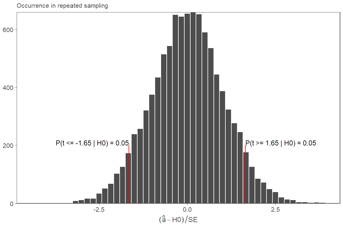
5. Additional t-test figure
This one is not in the paper. I used it for an internal Ph.D. seminar
t_dist <- data.frame(ps = rt(n=10000, df=n_obs-2))
test_stat <- 1.65
quant_test <- round(1 - pt(test_stat, df=n_obs-2), 2)

fZ <-
  ggplot(data=t_dist, aes(x=ps)) +
  geom_histogram(bins=50, color="white", fill="gray30") +
  geom_segment(color="red",
               x=test_stat, y=0,
               xend=test_stat, yend=200) +
  geom_segment(color="red",
               x=-test_stat, y=0,
               xend=-test_stat, yend=200) +
  # geom_area(color=high_red, fill=high_red, alpha=0.5) +
  annotate("text", x=test_stat, y=200,
           size=3, hjust=0, vjust=0,
           label=paste0("P(t >= ", test_stat, " | H0) = ", quant_test)) +
  annotate("text", x=-test_stat, y=200,
           size=3, hjust=1, vjust=0,
           label=paste0("P(t <= -", test_stat, " | H0) = ", quant_test)) +
  scale_y_continuous(expand=c(0,0)) +
  labs(x = expression((hat(a)-H0)/SE),
       y = NULL,
       subtitle = "Occurrence in repeated sampling") +
  theme(legend.position = "none")
fZ
6. Fitting the Bayesian models
To fit a Bayesian model I use Stan, or, more precisely, its R bindings in cmdstanr. To fit a Bayesian model, we need to:
- Write the corresponding model using the Stan language
- Compile the code into a Stan model executable (an .exe file)
- Make a list of data to feed into the .exe file
- Let the model run and generate MCMC chains (or whatever algorithm is specified)
6.1 Bayesian model with diffuse/very weak priors
sample1 <- samples$data[[1]]
The following descriptive are useful when assessing what priors to use:
sample1_descs <- c(
  u_y = mean(sample1$y),
  u_x = mean(sample1$x),
  s_y = sd(sample1$y),
  s_x = sd(sample1$x)
)

round(sample1_descs, 3)
   u_y    u_x    s_y    s_x
 0.499 -0.060 20.638  1.092
The model itself is coded in the Stan language. There are many excellent tutorials on Stan available online. So I won’t waste space explaining it here. For various reasons (e.g., debugging) it is customary to put the model code in a separate .stan file. All the model files can be found in the /Stan/ folder of the repo.
cat(read_lines("../Stan/sim-vweak-priors.stan"), sep = "\n")
data{
  int<lower=1> N;
  real y[N];
  real x[N];
}
parameters{
  real a0;
  real a1;
  real<lower=0> sigma;
}
model{
  vector[N] mu;
  sigma ~ exponential( 1.0 / 21.0 );
  a0 ~ normal( 0 , 100 );
  a1 ~ normal( 0 , 100 );
  for ( i in 1:N ) {
    mu[i] = a0 + a1 * x[i];
  }
  y ~ normal( mu , sigma );
}Next, we compile the model to an .exe file
model_vweak_priors <- cmdstan_model("../Stan/sim-vweak-priors.stan")
Now, we prepare the list of data to feed into the model.
We run the model
fit_vweak_priors <- model_vweak_priors$sample(
  data = input_data,
  iter_sampling = 1000,
  iter_warmup = 1000,
  chains = 4,
  parallel_chains = 4,
  seed = 1234,
  refresh = 1000
)
Running MCMC with 4 parallel chains...

Chain 1 Iteration:    1 / 2000 [  0%]  (Warmup)
Chain 1 Iteration: 1000 / 2000 [ 50%]  (Warmup)
Chain 1 Iteration: 1001 / 2000 [ 50%]  (Sampling)
Chain 1 Iteration: 2000 / 2000 [100%]  (Sampling)
Chain 2 Iteration:    1 / 2000 [  0%]  (Warmup)
Chain 2 Iteration: 1000 / 2000 [ 50%]  (Warmup)
Chain 2 Iteration: 1001 / 2000 [ 50%]  (Sampling)
Chain 2 Iteration: 2000 / 2000 [100%]  (Sampling)
Chain 3 Iteration:    1 / 2000 [  0%]  (Warmup)
Chain 3 Iteration: 1000 / 2000 [ 50%]  (Warmup)
Chain 3 Iteration: 1001 / 2000 [ 50%]  (Sampling)
Chain 4 Iteration:    1 / 2000 [  0%]  (Warmup)
Chain 1 finished in 0.1 seconds.
Chain 2 finished in 0.1 seconds.
Chain 3 Iteration: 2000 / 2000 [100%]  (Sampling)
Chain 3 finished in 0.1 seconds.
Chain 4 Iteration: 1000 / 2000 [ 50%]  (Warmup)
Chain 4 Iteration: 1001 / 2000 [ 50%]  (Sampling)
Chain 4 Iteration: 2000 / 2000 [100%]  (Sampling)
Chain 4 finished in 0.1 seconds.

All 4 chains finished successfully.
Mean chain execution time: 0.1 seconds.
Total execution time: 0.6 seconds.
Here is the summary of the resulting posterior distribution of the model parameters
fit_vweak_priors$summary(variables = c("sigma", "a0", "a1")) |>
  mutate(across(where(is.numeric), round, 3)) |>
  kable()
| variable | mean | median | sd | mad | q5 | q95 | rhat | ess_bulk | ess_tail |
|---|---|---|---|---|---|---|---|---|---|
| sigma | 20.556 | 20.380 | 2.125 | 2.074 | 17.446 | 24.220 | 1.003 | 3094.064 | 2515.482 |
| a0 | 0.756 | 0.778 | 2.921 | 2.932 | -3.884 | 5.581 | 1.000 | 3366.030 | 2861.077 |
| a1 | 4.241 | 4.241 | 2.665 | 2.681 | -0.186 | 8.541 | 1.000 | 3496.024 | 2752.886 |
Posterior descriptives
This is one form of getting the mcmc chain output. We need the draws to draw inferences about the posterior.
postdraws_vweak_prior <- fit_vweak_priors$draws(format = "draws_df")
head(postdraws_vweak_prior)
# A draws_df: 6 iterations, 1 chains, and 4 variables
  lp__     a0   a1 sigma
1 -173  2.697  4.0    21
2 -174 -1.066  6.8    18
3 -173  0.071  5.6    19
4 -174  2.678  6.5    23
5 -174 -1.515  2.1    18
6 -176 -1.275 -2.1    23
# ... hidden reserved variables {'.chain', '.iteration', '.draw'}
The posterior 90% centered credible interval:
The posterior probability that a1 < 0:
emp_a1 <- ecdf(postdraws_vweak_prior$a1)
emp_a1(0)
[1] 0.058256.2. Bayesian model with weakly informative priors
This is basically the same model, just with different hard-coded priors.
cat(read_lines("../Stan/sim-wkinfo-priors.stan"), sep = "\n")
data{
  int<lower=1> N;
  real y[N];
  real x[N];
}
parameters{
  real a0;
  real a1;
  real<lower=0> sigma;
}
model{
  vector[N] mu;
  sigma ~ exponential( 1.0 / 21.0 );
  a0 ~ normal( 0 , 100 );
  a1 ~ normal( 0 , 4 );
  for ( i in 1:N ) {
    mu[i] = a0 + a1 * x[i];
  }
  y ~ normal( mu , sigma );
}
model_wkinfo_priors <- cmdstan_model("../Stan/sim-wkinfo-priors.stan")
Because we use the same data (The list input_data), we can fit the new model now:
fit_wkinfo_priors <- model_wkinfo_priors$sample(
  data = input_data,
  iter_sampling = 1000,
  iter_warmup = 1000,
  chains = 4,
  parallel_chains = 4,
  seed = 1234,
  refresh = 1000
)
Running MCMC with 4 parallel chains...

Chain 1 Iteration:    1 / 2000 [  0%]  (Warmup)
Chain 1 Iteration: 1000 / 2000 [ 50%]  (Warmup)
Chain 1 Iteration: 1001 / 2000 [ 50%]  (Sampling)
Chain 1 Iteration: 2000 / 2000 [100%]  (Sampling)
Chain 2 Iteration:    1 / 2000 [  0%]  (Warmup)
Chain 2 Iteration: 1000 / 2000 [ 50%]  (Warmup)
Chain 2 Iteration: 1001 / 2000 [ 50%]  (Sampling)
Chain 2 Iteration: 2000 / 2000 [100%]  (Sampling)
Chain 3 Iteration:    1 / 2000 [  0%]  (Warmup)
Chain 3 Iteration: 1000 / 2000 [ 50%]  (Warmup)
Chain 3 Iteration: 1001 / 2000 [ 50%]  (Sampling)
Chain 3 Iteration: 2000 / 2000 [100%]  (Sampling)
Chain 4 Iteration:    1 / 2000 [  0%]  (Warmup)
Chain 4 Iteration: 1000 / 2000 [ 50%]  (Warmup)
Chain 4 Iteration: 1001 / 2000 [ 50%]  (Sampling)
Chain 1 finished in 0.1 seconds.
Chain 2 finished in 0.1 seconds.
Chain 3 finished in 0.1 seconds.
Chain 4 Iteration: 2000 / 2000 [100%]  (Sampling)
Chain 4 finished in 0.1 seconds.

All 4 chains finished successfully.
Mean chain execution time: 0.1 seconds.
Total execution time: 0.3 seconds.
Here is the summary of the resulting posterior distribution of the model parameters
fit_wkinfo_priors$summary(variables = c("sigma", "a0", "a1")) |>
  mutate(across(where(is.numeric), round, 3)) |>
  kable()
| variable | mean | median | sd | mad | q5 | q95 | rhat | ess_bulk | ess_tail |
|---|---|---|---|---|---|---|---|---|---|
| sigma | 20.567 | 20.358 | 2.161 | 2.072 | 17.333 | 24.506 | 1.001 | 4276.167 | 3167.417 |
| a0 | 0.672 | 0.690 | 2.878 | 2.897 | -4.040 | 5.364 | 1.000 | 4199.116 | 2467.601 |
| a1 | 2.978 | 3.013 | 2.213 | 2.186 | -0.793 | 6.560 | 1.001 | 4074.289 | 3219.891 |
Posterior descriptives
The posterior 90% centered credible interval:
postdraws_wkinfo_prior <- fit_wkinfo_priors$draws(format = "draws_df")
quantile(postdraws_wkinfo_prior$a1, probs = c(0.05, 0.95))
        5%        95%
-0.7927523  6.5595845
The posterior probability that a1 < 0:
emp_a1 <- ecdf(postdraws_wkinfo_prior$a1)
emp_a1(0)
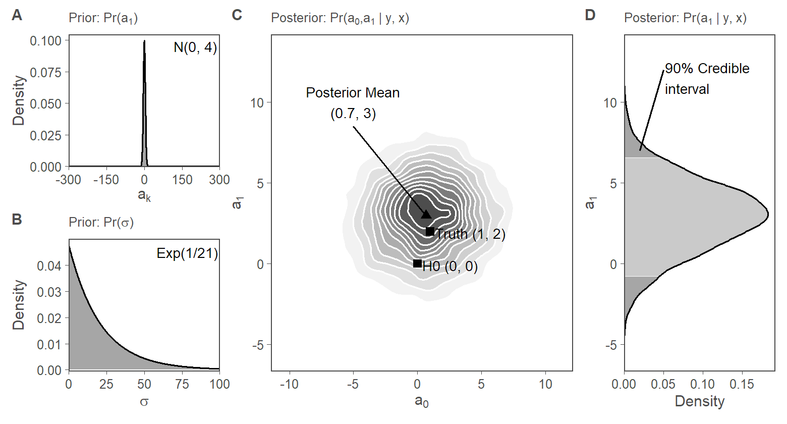
[1] 0.0927. Fig. 2: Visualization of Bayesian inference
7.1. Data preparations
The following code generates the density estimates, for the a1 posterior panels
# helper function for panel D
get_dens <- function(ppd, probs = c(0.05, 0.95)) {
  dens <- density(ppd)
  mode3 <- dens$x[dens$y == max(dens$y)]
  mode3.den <- dens$y[dens$x == mode3]
  dens.df <- data.frame(x = dens$x, y = dens$y)
  quantiles <- quantile(ppd, prob = probs)
  dens.df$quant <- factor(findInterval(dens.df$x, quantiles))
  dens.df$Q1 <- quantiles[1]
  dens.df$Q2 <- quantiles[2]
  return(dens.df)
}

post_dens <- get_dens(postdraws_vweak_prior$a1)
post_dens2 <- get_dens(postdraws_wkinfo_prior$a1)

max_dens <- max(c(post_dens$y, post_dens2$y))
The following code generates the density estimates, for the prior panels
x_length <- seq(-300, 300, length.out = 1000)
x_length2 <- seq(0, 100, length.out = 1000)
priors <- data.frame(
  a_den = dnorm(x = x_length, mean = 0, sd = 100),
  sigma_den = dexp(x = x_length2, rate = (1/21)),
  x1 = x_length,
  x2 = x_length2
)
priors2 <- data.frame(
  a_den = dnorm(x = x_length, mean = 0, sd = 4),
  sigma_den = dexp(x = x_length2, rate = (1/21)),
  x1 = x_length,
  x2 = x_length2
)

max_dens_a_prior <- max(c(priors$a_den, priors2$a_den))
Getting the plot ranges
7.2. Fig.2, Subfigure 1
f2.s1.panC <-
  ggplot(data = postdraws_vweak_prior, aes(x = a0, y = a1)) +
  stat_density_2d(aes(fill = ..level..), geom = "polygon", colour = "white") +
  annotate("point", x = 1, y = 2, color = "black", size = 2, shape = 15) +
  annotate("text", x = 1.4, y = 1.9, label = "Truth (1, 2)", hjust = 0, color = "black", size = 3) +
  annotate("point",
    x = mean(postdraws_vweak_prior$a0), y = mean(postdraws_vweak_prior$a1),
    color = "black", size = 2, shape = 17
  ) +
  annotate("text",
    x = -5, y = 10,
    label = paste0(
      "Posterior Mean\n(",
      round(mean(postdraws_vweak_prior$a0), 1),
      ", ",
      round(mean(postdraws_vweak_prior$a1), 1),
      ")"
    ),
    hjust = 0.5, color = "black", size = 3
  ) +
  annotate("segment",
    x = mean(postdraws_vweak_prior$a0), xend = -5,
    y = mean(postdraws_vweak_prior$a1), yend = 8.5
  ) +
  annotate("point", x = 0, y = 0, color = "black", size = 2, shape = 15) +
  annotate("text", x = 0.4, y = -0.1, label = "H0 (0, 0)", hjust = 0, color = "black", size = 3) +
  scale_x_continuous(expand = c(0, 0), limits = range_a0) +
  scale_y_continuous(expand = c(0, 0), limits = range_a1) +
  scale_fill_continuous(low = "grey95", high = "grey30") +
  theme(legend.position = "none") +
  labs(
    x = expression(a[0]),
    y = expression(a[1]),
    subtitle = quote("Posterior: Pr(" * a[0] * "," * a[1] * " | y, x)")
  )
f2.s1.panA <-
  ggplot(data = priors, aes(x = x1, y = a_den)) +
  geom_area(color = "black", fill = "grey30", alpha = 0.5) +
  scale_y_continuous(expand = expansion(mult = c(0.001, 0.05)), limits = c(0, max_dens_a_prior) ) +
  annotate("text", x = 290, y = 0.095, label = "N(0, 100)", hjust = 1, color = "black", size = 3) +
  scale_x_continuous(expand = c(0, 0), breaks = c(-300, -150, 0, 150, 300)) +
  labs(
    y = "Density",
    x = expression(a[k]),
    subtitle = quote("Prior: Pr(" * a[k] * ")")
  )
f2.s1.panB <-
  ggplot(data = priors, aes(x = x2, y = sigma_den)) +
  geom_area(color = "black", fill = "grey30", alpha = 0.5) +
  scale_y_continuous(expand = expansion(mult = c(0.01, 0.05))) +
  scale_x_continuous(expand = c(0, 0)) +
  annotate("text", x = 99, y = 0.045, label = "Exp(1/21)", hjust = 1, color = "black", size = 3) +
  labs(
    y = "Density",
    x = expression(sigma),
    subtitle = quote("Prior: Pr(" * sigma * ")")
  )
f2.s1.panD <-
  post_dens %>%
  ggplot(aes(x = x)) +
  geom_ribbon(aes(ymin = 0, ymax = y, fill = quant), alpha = 0.7) +
  geom_line(aes(y = y), color = "black") +
  labs(
    x = expression(a[1]),
    y = expression("Density"),
    subtitle = quote("Posterior: Pr(" * a[1] * " | y, x)")
  ) +
  scale_x_continuous(expand = c(0, 0)) +
  scale_y_continuous(expand = expansion(mult = c(0.0, 0.05))) +
  scale_fill_manual(values = c("grey50", "grey70", "grey50")) +
  theme(legend.position = "None") +
  annotate("segment", x = 7, xend = 12, y = 0.02, yend = 0.05) +
  annotate("text", x = 11.5, y = 0.052, label = "90% Credible\ninterval", color = "black", size = 3, hjust = 0) +
  coord_flip(xlim = range_a1, ylim = c(0, max_dens))

layout <- "
ACCD
BCCD
"

fig2.s1 <- f2.s1.panA + f2.s1.panB + f2.s1.panC + f2.s1.panD +
  plot_layout(design = layout) +
  plot_annotation(tag_levels = "A")
7.3. Fig.2, Subfigure 2
f2.s2.panC <-
  ggplot(data = postdraws_wkinfo_prior, aes(x = a0, y = a1)) +
  stat_density_2d(aes(fill = ..level..), geom = "polygon", colour = "white") +
  annotate("point", x = 1, y = 2, color = "black", size = 2, shape = 15) +
  annotate("text", x = 1.4, y = 1.9, label = "Truth (1, 2)", hjust = 0, color = "black", size = 3) +
  annotate("point",
    x = mean(postdraws_wkinfo_prior$a0), y = mean(postdraws_wkinfo_prior$a1),
    color = "black", size = 2, shape = 17
  ) +
  annotate("text",
    x = -5, y = 10,
    label = paste0(
      "Posterior Mean\n(",
      round(mean(postdraws_wkinfo_prior$a0), 1),
      ", ",
      round(mean(postdraws_wkinfo_prior$a1), 1),
      ")"
    ),
    hjust = 0.5, color = "black", size = 3
  ) +
  annotate("segment",
    x = mean(postdraws_wkinfo_prior$a0), xend = -5,
    y = mean(postdraws_wkinfo_prior$a1), yend = 8.5
  ) +
  annotate("point", x = 0, y = 0, color = "black", size = 2, shape = 15) +
  annotate("text", x = 0.4, y = -0.1, label = "H0 (0, 0)", hjust = 0, color = "black", size = 3) +
  scale_x_continuous(expand = c(0, 0), limits = range_a0) +
  scale_y_continuous(expand = c(0, 0), limits = range_a1) +
  scale_fill_continuous(low = "grey95", high = "grey30") +
  theme(legend.position = "none") +
  labs(
    x = expression(a[0]),
    y = expression(a[1]),
    subtitle = quote("Posterior: Pr(" * a[0] * "," * a[1] * " | y, x)")
  )
f2.s2.panA <-
  ggplot(data = priors2, aes(x = x1, y = a_den)) +
  geom_area(color = "black", fill = "grey30", alpha = 0.5) +
  scale_y_continuous(expand = expansion(mult = c(0.001, 0.05)), limits = c(0, max_dens_a_prior)) +
  annotate("text", x = 290, y = 0.095, label = "N(0, 4)", hjust = 1, color = "black", size = 3) +
  scale_x_continuous(expand = c(0, 0), breaks = c(-300, -150, 0, 150, 300)) +
  labs(
    y = "Density",
    x = expression(a[k]),
    subtitle = quote("Prior: Pr(" * a[1] * ")")
  )
f2.s2.panB <-
  ggplot(data = priors2, aes(x = x2, y = sigma_den)) +
  geom_area(color = "black", fill = "grey30", alpha = 0.5) +
  scale_y_continuous(expand = expansion(mult = c(0.01, 0.05))) +
  scale_x_continuous(expand = c(0, 0)) +
  annotate("text", x = 99, y = 0.045, label = "Exp(1/21)", hjust = 1, color = "black", size = 3) +
  labs(
    y = "Density",
    x = expression(sigma),
    subtitle = quote("Prior: Pr(" * sigma * ")")
  )
f2.s2.panD <-
  post_dens2 %>%
  ggplot(aes(x = x)) +
  geom_ribbon(aes(ymin = 0, ymax = y, fill = quant), alpha = 0.7) +
  geom_line(aes(y = y), color = "black") +
  labs(
    x = expression(a[1]),
    y = expression("Density"),
    subtitle = quote("Posterior: Pr(" * a[1] * " | y, x)")
  ) +
  scale_x_continuous(expand = c(0, 0), limits = range_a1) +
  scale_y_continuous(expand = expansion(mult = c(0.0, 0.05))) +
  scale_fill_manual(values = c("grey50", "grey70", "grey50")) +
  theme(legend.position = "None") +
  annotate("segment", x = 7, xend = 12, y = 0.02, yend = 0.05) +
  annotate("text", x = 11.5, y = 0.052, label = "90% Credible\ninterval", color = "black", size = 3, hjust = 0) +
  coord_flip(xlim = range_a1, ylim = c(0, max_dens))

layout <- "
ACCD
BCCD
"

fig2.s2 <- f2.s2.panA + f2.s2.panB + f2.s2.panC + f2.s2.panD +
  plot_layout(design = layout) +
  plot_annotation(tag_levels = "A")
fig2.s1

fig2.s2
Saving subfigures
save_fig(fig=fig2.s1, figname = "fig2-1", w = 6.2, h = 3.3)
save_fig(fig=fig2.s2, figname = "fig2-2", w = 6.2, h = 3.3)
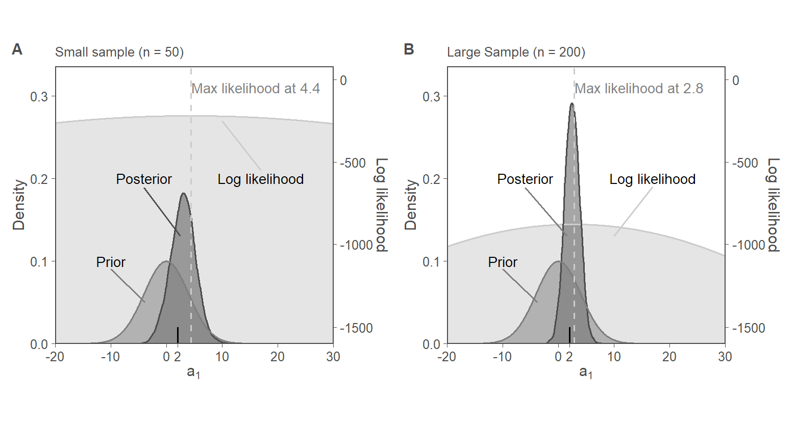
8. Fig. 3: Priors vs Likelihood
8.1. Generate a larger sample
8.2. Fitting the weakly informative model to larger sample
fit_wkinfo_priors_large <- model_wkinfo_priors$sample(
  data = input_data2,
  iter_sampling = 1000,
  iter_warmup = 1000,
  chains = 4,
  parallel_chains = 4,
  seed = 1234,
  refresh = 1000
)
Running MCMC with 4 parallel chains...

Chain 1 Iteration:    1 / 2000 [  0%]  (Warmup)
Chain 1 Iteration: 1000 / 2000 [ 50%]  (Warmup)
Chain 1 Iteration: 1001 / 2000 [ 50%]  (Sampling)
Chain 2 Iteration:    1 / 2000 [  0%]  (Warmup)
Chain 2 Iteration: 1000 / 2000 [ 50%]  (Warmup)
Chain 2 Iteration: 1001 / 2000 [ 50%]  (Sampling)
Chain 3 Iteration:    1 / 2000 [  0%]  (Warmup)
Chain 3 Iteration: 1000 / 2000 [ 50%]  (Warmup)
Chain 3 Iteration: 1001 / 2000 [ 50%]  (Sampling)
Chain 4 Iteration:    1 / 2000 [  0%]  (Warmup)
Chain 1 Iteration: 2000 / 2000 [100%]  (Sampling)
Chain 1 finished in 0.2 seconds.
Chain 2 Iteration: 2000 / 2000 [100%]  (Sampling)
Chain 2 finished in 0.1 seconds.
Chain 3 Iteration: 2000 / 2000 [100%]  (Sampling)
Chain 3 finished in 0.1 seconds.
Chain 4 Iteration: 1000 / 2000 [ 50%]  (Warmup)
Chain 4 Iteration: 1001 / 2000 [ 50%]  (Sampling)
Chain 4 Iteration: 2000 / 2000 [100%]  (Sampling)
Chain 4 finished in 0.1 seconds.

All 4 chains finished successfully.
Mean chain execution time: 0.1 seconds.
Total execution time: 0.3 seconds.
postdraws_wkinfo_prior_large <- fit_wkinfo_priors_large$draws(format = "draws_df")
fit_wkinfo_priors_large$summary(variables = c("sigma", "a0", "a1")) |>
mutate(across(where(is.numeric), round, 3)) |>
kable()
| variable | mean | median | sd | mad | q5 | q95 | rhat | ess_bulk | ess_tail |
|---|---|---|---|---|---|---|---|---|---|
| sigma | 19.649 | 19.617 | 0.988 | 1.000 | 18.088 | 21.313 | 0.999 | 4670.806 | 2760.187 |
| a0 | -0.136 | -0.149 | 1.383 | 1.358 | -2.424 | 2.125 | 1.001 | 3777.942 | 2872.741 |
| a1 | 2.467 | 2.467 | 1.324 | 1.337 | 0.317 | 4.634 | 1.000 | 3953.647 | 3027.360 |
8.3. Collecting Prior, likelihood, posterior for small, current sample
ols_model_small <- lm(y ~ x, data = sample1)
a0 <- ols_model_small$coefficients[["(Intercept)"]]
usd <- sd(ols_model_small$residuals)
a1_hat <- ols_model_small$coefficients[["x"]]

small_sample_data <- tibble(a1 = seq(-20, +30, length.out = 1000))
small_sample_data$loglik <- map_dbl(
  small_sample_data$a1,
  loglik_a1,
  x = sample1$x,
  y = sample1$y,
  a0 = a0,
  u_sd = usd
)
small_sample_data <-
  small_sample_data %>%
  mutate(
    # norm_lik = -2 * loglik, #exp(loglik) / sum(exp(loglik)),
    norm_lik = (loglik),
    prior = dnorm(a1, 0, 4),
    post = approxfun(density(postdraws_wkinfo_prior$a1))(a1)
  )
small_sample_data$post[is.na(small_sample_data$post)] <- 0
8.4. Collecting Prior, likelihood, posterior for larger sample
ols_model_large <- lm(y ~ x, data = sample2)
a0 <- ols_model_large$coefficients[["(Intercept)"]]
usd <- sd(ols_model_large$residuals)
a1_hat_big <- ols_model_large$coefficients[["x"]]

large_sample_data <- tibble(a1 = seq(-20, +30, length.out = 1000))
large_sample_data$loglik <- map_dbl(
  large_sample_data$a1,
  loglik_a1,
  x = sample2$x,
  y = sample2$y,
  a0 = a0,
  u_sd = usd
)
large_sample_data <-
  large_sample_data %>%
  mutate(
    # norm_lik = -2 * loglik, #exp(loglik) / sum(exp(loglik)),
    norm_lik = (loglik),
    prior = dnorm(a1, 0, 4),
    post = approxfun(density(postdraws_wkinfo_prior_large$a1))(a1)
  )
large_sample_data$post[is.na(large_sample_data$post)] <- 0
8.5. Fig. 3, Panel A and Panel B
SCALER_1 <- -2 * 0.0001
f3.panA <-
  small_sample_data %>%
  mutate(norm_lik = (-1600 - norm_lik) * SCALER_1) %>%
  pivot_longer(c(norm_lik, prior, post), names_to = "part") %>%
  ggplot(aes(x = a1, y = value, group = part, color = part, fill = part)) +
  geom_ribbon(aes(ymin = 0, ymax = value), alpha = 0.5) +
  geom_line() +
  geom_vline(xintercept = a1_hat, color = "grey80", linetype = "dashed") +
  labs(
    y = "Density",
    x = expression(a[1]),
    subtitle = "Small sample (n = 50)"
  ) +
  annotate("text",
    x = c(-10, -4, 17),
    y = c(0.1, 0.2, 0.20),
    label = c("Prior", "Posterior", "Log likelihood"),
    hjust = 0.5,
    size = 3
  ) +
  annotate("segment",
    x = c(-10, -4, 17),
    y = c(0.090, 0.189, 0.21),
    xend = c(-3.8, 2.5, 10),
    yend = c(0.050, 0.13, 0.27),
    color = c("grey50", "grey30", "grey80")
  ) +
  annotate("text",
    x = a1_hat + 0.1,
    y = 0.31, label = paste("Max likelihood at", round(a1_hat, 1)),
    hjust = 0, color = "grey50", size = 3
  )


f3.panB <-
  large_sample_data %>%
  mutate(norm_lik = (-1600 - norm_lik) * SCALER_1) %>%
  pivot_longer(c(norm_lik, prior, post), names_to = "part") %>%
  ggplot(aes(x = a1, y = value, group = part, color = part, fill = part)) +
  geom_ribbon(aes(ymin = 0, ymax = value), alpha = 0.5) +
  geom_line() +
  geom_vline(xintercept = a1_hat_big, color = "grey80", linetype = "dashed") +
  labs(
    y = "Density",
    x = expression(a[1]),
    subtitle = "Large Sample (n = 200)"
  ) +
  annotate("text",
    x = c(-10, -6, 17),
    y = c(0.1, 0.2, 0.20),
    label = c("Prior", "Posterior", "Log likelihood"),
    hjust = 0.5,
    size = 3
  ) +
  annotate("segment",
    x = c(-10, -6, 17),
    y = c(0.090, 0.189, 0.19),
    xend = c(-3.8, 1.5, 10),
    yend = c(0.050, 0.13, 0.13),
    color = c("grey50", "grey50", "grey80")
  ) +
  annotate("text",
    x = a1_hat_big + .1,
    y = 0.31, label = paste("Max likelihood at", round(a1_hat_big, 1)),
    hjust = 0, color = "grey50", size = 3
  )

fig3 <-
  f3.panA + f3.panB +
  plot_annotation(tag_levels = "A") &
  annotate("segment", x = 2, y = 0, xend = 2, yend = 0.02) &
  theme(legend.position = "none", aspect.ratio=1) &
  scale_color_manual(values = c("grey80", "grey30", "grey50")) &
  scale_fill_manual(values = c("grey80", "grey30", "grey50")) &
  scale_y_continuous(
    expand = expansion(mult = c(0, 0.05)),
    limits = c(0, 0.32),
    sec.axis = sec_axis(~ -1600 - . / SCALER_1, name = "Log likelihood")
  ) &
  scale_x_continuous(
    breaks = c(-20, -10, 0, 2, 10, 20, 30),
    expand = expansion(mult = c(0, 0))
  )
fig3
Saving figure
save_fig(fig=fig3, figname = "fig3", w = 6.2, h = 3.1)