2 Decision-Making Basics
2.1 Learning goals
- Introduce, apply, and evaluate a template for making data-driven decisions
- Highlight the importance of connecting analysis goals to decision-making goals
- Introduce a taxonomy of different types of analyses based on the type of questions that can be answered
- Discuss mental patterns useful for critically evaluating analyses and reducing analysis errors
2.2 Rational decision-making
As stated in Chapter 1, this course teaches you sensible decision-making with data. Before we dive into data analysis, it is useful to introduce the basics of economic decision theory. Not because we want to estimate and compute expected utility values—far from it—but because decision theory is a handy framework to guide our thinking. It provides a useful vocabulary to describe the issues we will tackle. It is useful for structuring complex problems and for reasoning about where the difficulty of a given decision problem is. We will use the following structure throughout the course. It allows us to apply our data analysis skills more effectively.
Decision theory asks how people “should” make decisions when uncertain about the consequences of their actions. The standard answer is: Maximize expected utility.1
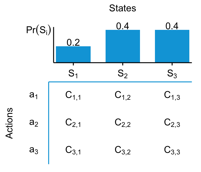
To calculate expected utility, we would need to:
- Enumerate all our possible actions \(a_i\)
- Enumerate all the possible future scenarios (often called ‘states’) \(S_k\)
- Assign probabilities of a future scenario occurring
- Connect each action \(a_i\) to a consequence \(C_{ik}\) if scenario \(S_k\) materializes
We can summarize these steps via a decision matrix, as in Figure 2.1:
If \(C_{i,k}\) is expressed in units of utility already, this matrix contains everything we need to know. For each row, we can compute an expected utility for that action. Then, we chose the action with the highest expected utility. For example the expected consequence \(\mathbb{E}\left[C_1\right]\) of taking action \(a_1\) is simply the sum of each scenario’s consequence of taking that action weighted by how probable that scenario is: \(\mathbb{E}\left[C_1\right] = 0.2 * C_{1,1} + 0.4 * C_{1,2} + 0.4 * C_{1,3}\). Let’s put in some numbers and calculate:
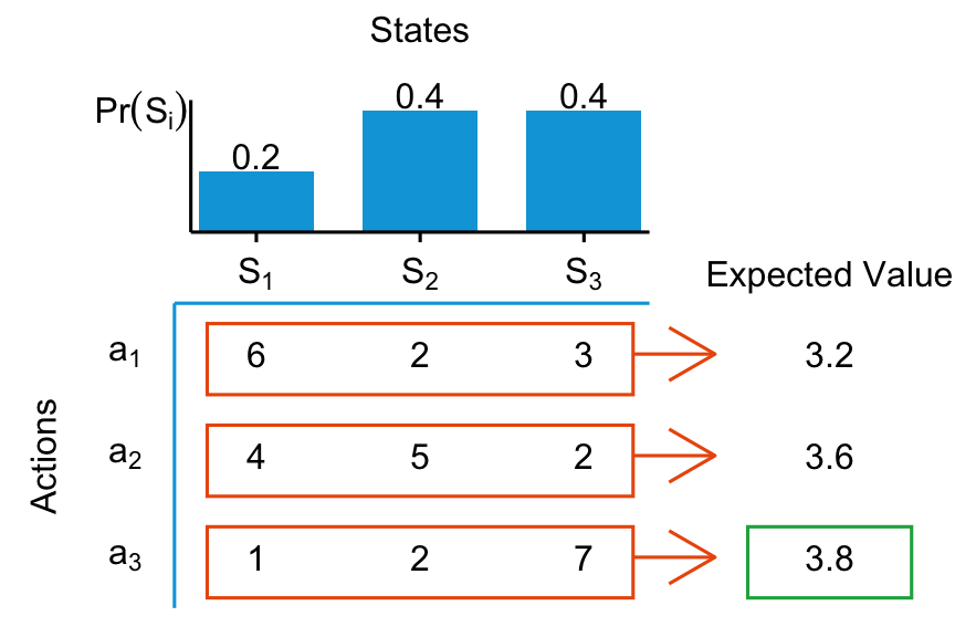
Here the expected value of chosing action \(a_3\) is the highest, hence we should choose \(a_3\). If only real decision-making were that easy! We abstracted from many real-world implementation issues. For example, how can we specify a utility function? And how do we quantify probabilities for each scenario? What are these scenarios in the first place? Aren’t there infinitely many scenarios? And what about actions? Whose “expectations” are we maximizing? Yours? What if it is a team decision? Thus, it is often infeasible to specify all that is needed for standard utility maximization for many real-world applications. However, decision theory is still useful as a framework. We want to think of decisions as choosing an action and that actions can lead to different consequences, depending on what will happen in the future. Actions can be good or bad depending on which scenario will happen. We always want to be mindful of the fact that we are uncertain about which scenario will materialize.
2.3 Decision-making, data, and uncertainty
Decision matrices are handy because they highlight the role of uncertainty. The first thing to note is that most important business decisions involve some degree of uncertainty. Think of uncertainty simply as limited knowledge about past, present, or future events (Walker, Lempert, and Kwakkel 2013). The knowledge that you would need in order to choose the best action under various potential scenarios.
We want to structure any important decision process to take uncertainty into account. Here is where data analysis comes in. Dealing with uncertainty is crucial. We want to reduce it as best as possible and then deal with the remainder. And not all uncertainty is the same. For example, the following decisions are ordered in increasing magnitude of complexity, mostly because the uncertainty about future scenarios/states increases:2
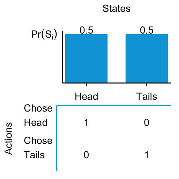
- I will toss a coin into the air. You guess heads or tails while the coin is in the air. you win $1 if you guess correctly. Which side do you choose?
- We can sell goods on credit. We have a large history of past transactions. Should we offer a new customer credit?
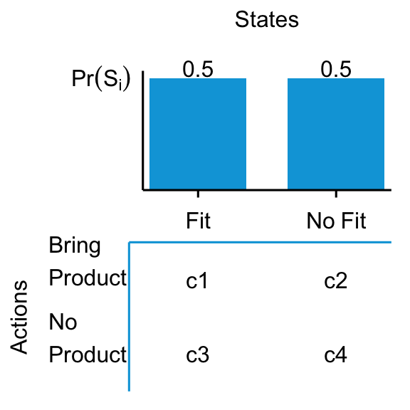
- We are designing a product for a new market. Matching customer taste matters most. How should we design the product?
- We are thinking about expanding our business to a new geographic market. That market has a chance of experiencing a protracted armed conflict within four years. Should we enter that market?
- Whether the market entrance will be successful depends on how the incumbent players react to our entrance. Should we enter that market?
What is different across these questions? There are two major sources of uncertainty in those examples, and they become more difficult going from question 1 to question 5. The first concerns uncertainty about future scenarios, the second concerns establishing what the outcome of an action in a given scenario is.
The coin toss in Q1 is a straightforward decision: it does not matter what you choose. You know the outcomes of each action, and the probability of each scenario happening is also well described by 50/50. You can compute that both actions are equivalent in expectations.
Question Q2, whether to sell on credit or not, is a bit more complicated, but not much. Assuming we can reasonably infer the probability of not collecting on a new customer from prior transactions (e.g., based on customer characteristics), we can also quantify the probability of the relevant states and the potential consequences. Again, we can compute what action is best in expectations.

Question Q3, whether to bring the product to market, is more complex. Both inputs, scenario probabilities and the consequences, are hard to reason about and, hence, to quantify. It is harder to quantify the probabilities of each scenario because there is not enough historical data from which to infer stable probabilities (it’s a new product / new market). The same goes for the consequences. In fact, one of the most difficult thing in settin up decision matrices is to properly disentangly actions from scenarios. Scenarios are independent of actions. we could for example, envision different scenarios of number of consumers with a taste fit and map the actions enter / not enter to outcomes based on the number of consumers. But this is not the only way to structure this problem. We need to make some assumptions—form a mental model—about customer preferences and behavior, or we get stuck here. Based on such a model, we can potentially find comparable situations and infer relevant data from those.
Question Q4 is even more complex. Whether an armed conflict will break out in four years is very difficult to reason about. It depends on the interplay of the actions of many players; every built-up to a conflict is different, so there is not much past data that can help us make accurate predictions four years into the future. We need to make decisions differently in such situations, and we will talk about how to do that later.
Finally, question Q5 is the most complex. It is a game theory problem, where the consequences of our actions not only depend on which scenario happens, but also on the actions of players who take our possible actions into account.
What have we learned form comparing the five questions? The difficulty of a decision often depends on the uncertainty surrounding it. Next, we will discuss how data analysis can help us dealing with uncertainty.
2.4 A stylized decision-making process
The decision-making matrices in the previous section illustrate what we need to know to make decisions: our available actions, relevant scenarios and how plausible they are, and finally consequences of each action in each scenario. We will use data analysis to collect these decision inputs as best as possible. However, it is easy to get stuck and stare at the data, not seeing the forest for the trees. Over the years of teaching and practicing data analysis in various forms, we have seen it happen frequently; to students at all levels–from bachelor to PhD students. It still happens to us too. The best remedy against getting stuck is to remind yourself where you are in the process and what the next important steps are. For that, you need to have a good process framework, though. So, let us try to give you one.
If you google “business decision-making” then you will at some point stumble upon a process similar to the one in Figure 2.6:

Figure 2.6 (based on Schoenfeld (2010)) shows our version of what a decision-making process looks like. While very stylized, this is not a bad schema for trying to find answers to important business problems. Let us explain each step in turn.3
2.4.1 Clarify the problem
This is the most important step and data analysis is an integral part of it. Here we clarify what we want to decide on and what we need to know for that decision. For example, say we are faced with declining sales (the problem) and we need to decide on a course of action to increase sales again (the decision). Which action is best will depend on what the cause is for the decrease in sales. Exploratory data analysis and confirmatory analysis (which we introduce later) are important tools that we will use at this stage. We will use the analysis to inform a mental model of the drivers of sales—the possible causes. This will be crucial for defining different scenarios/states later and mapping actions to outcomes.
It is key to slow down and properly identify a problem’s underlying mechanisms. Even for exploratory analyses, step back first and take a moment to go through the steps described in the previous paragraph. E.g., is the sales decline because of demotivated salespeople, or are salespeople demotivated because the product is outdated? If we don’t know which, can we do an analysis to figure it out? It can easily happen that we mistake symptoms for causes.
Often, we need to gather and analyze a significant amount of data to better understand what is happening. A lot of our data analysis will happen at this stage. Consider the following simple example.
You work for a technology vendor that sells software products bundled with support packages. The support packages are a big part of overall revenues. The company’s CFO comes to you and mentions that one client contacted her because he was unhappy and did not want to renew his support package. She asks you to look into whether there are any signs of issues with the company’s support offering. You reason that if there are issues with the support offering (a problem), you should find hints in the latest customer survey that you ran. You go and have a look at the main table:
| Responses | Percent | |
|---|---|---|
| Highly Likely | 796 | 49.9 |
| Likely | 350 | 22.0 |
| Maybe | 253 | 15.9 |
| Probably Not | 109 | 6.8 |
| Certainly Not | 86 | 5.4 |
| TOTAL | 1594 | 100 |
Table 2.1 seems to suggest that 12% of respondents indicate that they are “probably not” or “certainly not” renewing the service package. You know from experience that such survey answers often overstate the true dropout rate. Analyzing is comparing. You need a benchmark to judge whether there is an issue. You know that the numbers are in line with survey responses from previous years. So, you could go to the CFO and tell her that nothing seems to have changed.
But you do not do that yet. Your company has different support tiers. You know that customers are quite heterogeneous across tiers. So, you decide to split the survey responses by support tier. You are presented with the following data:
| Tier 1 | Tier 2 | Tier 3 | Tier 4 | Tier 5 | |
|---|---|---|---|---|---|
| Highly Likely | 218 | 212 | 163 | 111 | 92 |
| Likely | 79 | 74 | 78 | 61 | 58 |
| Maybe | 59 | 52 | 65 | 55 | 22 |
| Probably Not | 16 | 19 | 13 | 39 | 22 |
| Certainly Not | 24 | 15 | 7 | 11 | 29 |
| TOTAL | 396 | 372 | 326 | 277 | 223 |
You can see that most support tiers are fine. However, Table 2.2 shows that the high tiers (tiers 4 and 5 are the most expensive ones) have significantly higher frequencies of unhappy responses. You found a meaningful pattern.
This is a very simple example of what data analytics is all about finding meaningful patterns in raw data. (see Chapter 1). We will have much more to say about this in Chapter 3.
This pattern was not obvious in the overall survey answers in Table 2.1. The reason is that there are fewer responses for higher support tiers than for lower tiers. The unhappy higher tiers are underrepresented in the all-tier averages in Table 2.1. You create a quick visualization that shows the pattern more clearly. It is even more obvious in percentage terms (Figure 2.7):
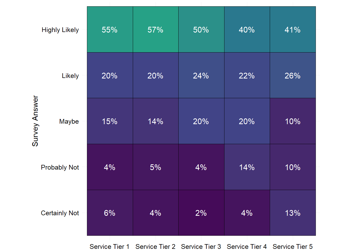
Stop for a moment and consider how you would have possibly spotted this pattern if you had not known it existed (an unknown unknown). How could you have found it? We used some expert knowledge (there are multiple Support Tiers, customers are heterogeneous across tiers, and tiers are not of equal size and importance). We also had the beginning of some type of mental model of the customers, which suggested that their satisfaction might vary across tiers (maybe higher tier customers are more demanding). Both led us to entertain the idea that mismatches might differ across tiers.

We point this out to highlight the importance of mental models. Only if you combine the right inquisitive mindset with a bit of background/expert knowledge will you be able to identify problems properly.
You probably do not want to stop right there, either. Before going to your boss to tell your CFO the bad news, you might want to understand better what is happening. In other words, we have a guiding question for the next analysis: What might be the reason for the low survey score for the expensive tiers? And how do we figure that out? Again, we now need to develop a mental model of how the customer response came to pass and start testing for indications that are either consistent or inconsistent with this model–rinse and repeat.
The general steps remain the same for all decision problems you might face. If you need to come up with a sales forecast, then “identifying the problem” becomes clarifying what you are supposed to forecast (e.g., all sales? product, service, and advertising? How far into the future? On a yearly or monthly basis?). Often the right answers to those questions can be found by asking a slightly different question–one of purpose. “What is the sales forecast for?”.
The previous example thus also illustrates the power of asking the right questions. One can structure a decision problem into a series of questions to be answered. Example questions for this stage of the process include:
- Who is doing what to whom?
- Where/When does the problem appear to arise?
- What is the process behind what we observe?
- What is the reason for the suspected reason?
- What do we need to solve this problem?
2.4.2 Establish decision criteria
To make good decisions, we need to know what goal we are working towards! Once we have clarified what the problem is, we should start defining criteria for what a good solution should look like. This is important to guide the analysis as we advance. We do not want to waste time and effort on analyses that turn out not decision-relevant.
It is hard to give good guidance here because these criteria are usually problem specific. For example, a sales forecast should have “expected accuracy” as a criterion to accept a forecast. But there are other potential criteria, too. Typical decision criteria considered are financial benefits, resource usage, quality, riskiness, acceptability to others, etc. In the case of the sales forecast, another criterion might be complexity. Are we willing to entertain forecasts based on hard-to-reason or even black-box machine learning models, or do we only entertain forecasts based on models we can reason about? This might be an important decision criterion depending on the cost of forecast errors and who will be held accountable for decisions based on the forecast.
Actions might have more than one outcome dimension. The mental model of “what drives what?” might also give insights into relevant criteria to consider. (Figure 2.6) If more than one matters, we need to weigh them too. You might have seen “decision matrices” like Figure 2.9 in practice. They are not strcitly decision matrices by our definition because they do not feature different scenarios and are thus ill-equipped to illustrate uncertainty.
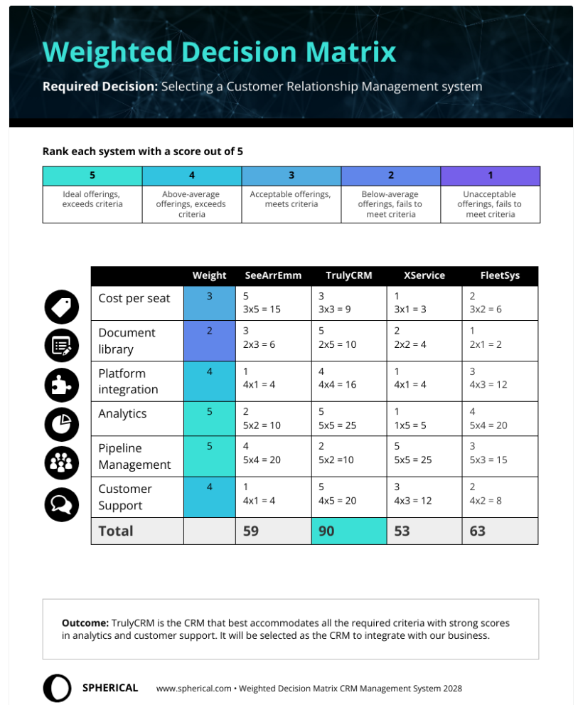
What Figure 2.9 illustrates well is that if there are multiple criteria, it is important to discuss how to weigh them. Multi-criteria decision-making is not an easy topic, because the notion of a “best solution” becomes non-trivial (Pomerol and Barba-Romero 2000; Aruldoss, Lakshmi, and Venkatesan 2013). It is not always obvious what the right weights should be. Because of time constraints and scope, we won’t go into much detail here. But we want to raise awareness for the issue and cover some simpler examples.
Typical questions you might want to ask yourself at this stage:
- What is affected by the possible alternatives?
- What do we need to trade off (e.g., costs versus benefits)?
- What cost is more significant for us?
2.4.3 List possible actions
After clarifying the problem and setting our decision criteria, we can start listing possible courses of action that might lead to a solution to the problem at hand.
Creativity is often key here. The insights gathered from a careful root-cause analysis in Step 1: “clarify the problem” are usually very useful at this stage too. Again, these should be condensed into our mental model (Figure 2.6). Developing alternative solutions often involves building and entertaining different mental models of how the problem might have arisen. Sometimes, this is done in brainstorming sessions with the whole team. Imagine you are part of a team, and some team members disagree on what the best course of action is. In some cases (e.g., enough resources), it might be the best way forward to analyze both courses in parallel until one alternative clearly dominates.
2.4.4 Evaluate possible actions
Creativity coaches often recommend listing ideas first and only evaluating them as to their feasibility, etc., later. This step is about two connected issues. Given our list of actions, we need to define clear scenarios and reason about their probabilities. At the same time, we need to map each action in our list of actions to consequences for each scenario. We need our mental model for both steps. Usually, we have started building it in Step 1, “clarifying the problem.” It becomes crucial now.
This is the second step where data analysis is often crucial:
- Are the mental models on which the solutions/actions are resting supported by the data? We must collect and analyze data to evaluate the assumptions underlying the solutions/actions. This is often called diagnostic analysis and the topic of Chapter 4.
- Properly fleshed-out solutions mapping actions to consequences often require data-based inputs and serious analysis.
Consider the following simple example of evaluating actions using data: imagine you are working for a supermarket chain. You are considering expansion strategies, and your job is to choose the next location. Each possible location is a different action. You decided the potential market size at a new location is a key decision criterion. So, right now, you are forecasting the potential sales of a new supermarket if it were opened at a specific, new location \(X_1\). There is no historical data because the chain has never had a store at that location \(X_1\). Let’s further assume it was decided that there is only a limited budget for external data, and good solutions need to be transparent in their reasoning. How would you go about this?
You have internal data on the other 140 supermarkets the firm runs. You can, for example, extract a table like this from the company databases:
| Market ID | Market size (m2) | No. Clients | Revenues (€) |
|---|---|---|---|
| 1 | 1,000 | 378,040 | 4,536,480 |
| 2 | 800 | 300,395 | 1,501,975 |
| 3 | 1,200 | 431,667 | 2,158,335 |
| 4 | 800 | 337,552 | 4,050,624 |
| 5 | 800 | 512,045 | 3,584,315 |
| 6 | 1,000 | 670,372 | 8,044,464 |
| 7 | 1,400 | 406,762 | 5,694,668 |
| 8 | 800 | 278,441 | 2,227,528 |
| 9 | 1,000 | 315,310 | 3,783,720 |
| 10 | 1,000 | 540,726 | 8,110,890 |
You know that the location available is ca. 1,200 square meters. That is one reason why your firm is considering setting up shop in that town. You could start by looking at what supermarkets of that size in your portfolio produce in revenues. You start by computing some average statistics:
| Size Group (sqm) | N | Avg. | SD | 5% Perc. | 95% Perc. |
|---|---|---|---|---|---|
| 700 | 16 | 4,874T€ | 3,326T€ | 1,944T€ | 10,849T€ |
| 800 | 26 | 4,184T€ | 3,409T€ | 1,417T€ | 10,833T€ |
| 1000 | 44 | 5,716T€ | 3,626T€ | 1,670T€ | 11,937T€ |
| 1200 | 29 | 5,674T€ | 3,098T€ | 1,811T€ | 10,550T€ |
| 1400 | 25 | 5,911T€ | 2,426T€ | 2,720T€ | 9,837T€ |
You know that the location available is ca. 1,200 square meters. That is one reason why your firm is considering setting up shop in that town. You could start by looking at what supermarkets of that size in your portfolio produce in revenues. You start by computing some average statistics:
The averages (means) are roughly as expected, with bigger stores having more revenues. But not always. The 29 1,200 square meter supermarkets have, on average, lower revenues than the 1,000 square meter markets.
Does it make sense to only report the mean of 5,674T€ as an estimate of the new market’s revenues? Probably not. The other columns in Table 2.4 give us an indication of the variation among the 1,200 square meter markets. The standard deviation (SD) measures how dispersed the data is relative to the mean. The SD of 3,098T€, circa 3 million euros, is large for a “standard” distance from the mean. We also notice significant variation when examining the 5% and 95% percentiles. They tell us that 5% of the 29 markets have revenues lower than 1,8 million euros and 5% higher than 10,5 million euros.4. The important point is that the three descriptives (SD, 5%, and 95% percentiles) show that there is a lot of variation around the mean. That tells us that the mean of similarly sized supermarkets likely is not a good forecast. Given the range of sales figures for this size category, the mean will likely be quite inaccurate.
We learned from the data that we cannot just look at similarly sized supermarkets we already have. What alternatives do we have? We now need to start entertaining some mental models. You often do this implicitly, but we want to highlight the importance of doing this more explicitly. The question we want to start with when building a model is: What would a process look like that generates the outcome we are interested in? (In this case, supermarket revenues). Such a model is also sometimes called a “data-generating process”. We can start simple. We could split revenues into two determinants: the number of customers served times the average basket size of their shopping (volume times price). Then, we think about the possible determinants of these two determinants. What would determine the average basket size? The average basket size is probably determined by the average wealth of the customers (assumption: wealthier customers buy more expensive products) and the amount they buy. Many things can drive the latter. Is the average wealthy customer someone who eats a lot outside and only buys small quantities? Or do they buy for a whole family, etc.? Another thing to consider is: What would determine how many customers shop in that location? The market size probably plays a role (customers are more likely to find what you are looking for). Also, the proximity of the market to where customers live. In that case, stores in densely populated areas should have more customers. On the other hand, it is more difficult and more expensive to find a large location for a store in densely populated areas. Thus, there should also be a negative relation between market size and population density in an area. We often like to draw DAGs (directed acyclical graphs) to visualize the data-generating process we have in mind. Figure 2.10 shows one describing our reasoning thus far.
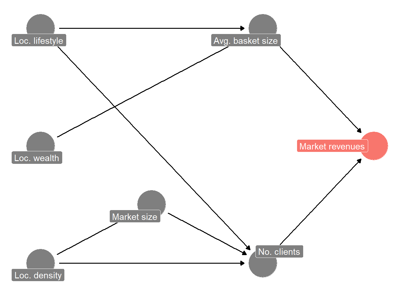
Figure 2.10 describes our reasoning in a simplified process graph. The node “Loc. lifestyle” is a catch-all for things like family shopping, commuting frequency, and other things affecting shopping behavior. For example, consultants jet-setting through the country most of the week will probably not buy many items but more expensive ones. For now, we just put a node like this in, rather than expanding our thinking on how lifestyle affects shopping behavior.
Often, visualizing your mental model helps you inspect it. Is our reasoning sound? Have we forgotten anything important? Probably. For example, we do not have competition from other supermarkets in the area in our model. Still, starting simple and adding more detail later is often better.
We want to test how descriptive this model is for the true data-generating process. If it can explain a decent part of the variation that we have observed in the revenues of supermarkets of the same size (Table 2.4), then it could give us very helpful guidance on making better predictions.
How can we test the model’s descriptive power? We are going into much more detail on how to do this when discussing predictive analytics in Chapter 5. But you can often get a decent idea with some simple descriptives. You have old data on the population density from previous planning projects readily at hand. It is sorted into categories, though. Still, we can expand our descriptive statistics and see how much variation within size and density groups exists:
| Groups: Size (sqm) x Density | N | Avg. | SD | 5% Perc. | 95% Perc. |
|---|---|---|---|---|---|
| 1200 x A | 6 | 4,095T€ | 2,236T€ | 1,418T€ | 6,658T€ |
| 1200 x B | 5 | 4,326T€ | 1,779T€ | 2,390T€ | 6,490T€ |
| 1200 x C | 6 | 5,844T€ | 2,602T€ | 3,459T€ | 9,561T€ |
| 1200 x D | 2 | 5,347T€ | 3,995T€ | 2,805T€ | 7,890T€ |
| 1200 x E | 10 | 7,258T€ | 3,826T€ | 3,033T€ | 12,943T€ |
Compared to the within-group variation shown in Table 2.4, Table 2.5 shows that we already do a better job by also considering density in the area as a determinant of revenues. The variation across density categories shows itself in the variation across averages and is sizable (compare it to the mean of 5,674T€ for the 1,200 sqm supermarkets). We only focus on the relevant size category (1,200 square meters) here for ease of exposition, but you should always check whether your model holds for all areas of the data. The standard deviation and percentiles still indicate a sizable amount of variation though. If we can further increase the explained variation, it would be worthwhile to do so.
Let’s assume you also have categories of how wealthy people are on average in the area around the supermarket. These are also from previous planning projects (never throw away data). We can also expand our descriptives via this potential determinant:
| Groups: Size (sqm) x Wealth | N | Avg. | SD | 5% Perc. | 95% Perc. |
|---|---|---|---|---|---|
| 1200 x A | 6 | 2,283T€ | 715T€ | 1,418T€ | 3,065T€ |
| 1200 x B | 5 | 4,271T€ | 953T€ | 3,295T€ | 5,238T€ |
| 1200 x C | 13 | 6,407T€ | 1,927T€ | 4,105T€ | 9,295T€ |
| 1200 x D | 4 | 7,792T€ | 2,994T€ | 4,616T€ | 10,536T€ |
| 1200 x E | 1 | 15,021T€ | NA | 15,021T€ | 15,021T€ |
Table 2.6 shows that wealth also sorts well within the size category of 1,200 square meter markets in our portfolio. You can even combine all our splits and expand your descriptives by a three-way-split:
| Groups: Size (sqm) x Density x Wealth | N | Avg. | SD | 5% Perc. | 95% Perc. |
|---|---|---|---|---|---|
| 1200 x A x A | 2 | 1,472T€ | 153T€ | 1,375T€ | 1,569T€ |
| 1200 x A x C | 3 | 5,768T€ | 1,176T€ | 4,735T€ | 6,849T€ |
| 1200 x A x D | 1 | 4,319T€ | — | 4,319T€ | 4,319T€ |
| 1200 x B x A | 1 | 2,158T€ | — | 2,158T€ | 2,158T€ |
| 1200 x B x B | 1 | 3,315T€ | — | 3,315T€ | 3,315T€ |
| 1200 x B x C | 3 | 5,386T€ | 1,335T€ | 4,291T€ | 6,660T€ |
| 1200 x C x B | 1 | 3,290T€ | — | 3,290T€ | 3,290T€ |
| 1200 x C x C | 3 | 4,941T€ | 893T€ | 4,083T€ | 5,659T€ |
| 1200 x C x D | 2 | 8,474T€ | 3,075T€ | 6,517T€ | 10,431T€ |
| 1200 x D x A | 1 | 2,523T€ | — | 2,523T€ | 2,523T€ |
| 1200 x D x C | 1 | 8,172T€ | — | 8,172T€ | 8,172T€ |
| 1200 x E x A | 2 | 3,038T€ | 77T€ | 2,989T€ | 3,087T€ |
| 1200 x E x B | 3 | 4,917T€ | 502T€ | 4,422T€ | 5,249T€ |
| 1200 x E x C | 3 | 8,943T€ | 1,310T€ | 7,938T€ | 10,218T€ |
| 1200 x E x D | 1 | 9,902T€ | — | 9,902T€ | 9,902T€ |
| 1200 x E x E | 1 | 15,021T€ | — | 15,021T€ | 15,021T€ |
Now, Table 2.7 has started to become unwieldy. But the combo density x wealth of the area seems important. The variation in means has increased, and the standard deviation decreased. These are signs we might be able to explain a lot of variation in revenues with these three features. We are computing conditional means here. Means conditional on a given size, density, and wealth level. As we will see in later chapters, regression models and other machine learning approaches essentially do what we did here—only more sophisticated. More sophisticated models estimate means (or other statistics) conditional on many possible conditions. The important takeaway here is to realize that we often want to know conditional means in forecasting problems. As you can see, we can do this to some rudimentary degree just by using tables.
We have a problem though: sample size. While it looks like the combo size x density x wealth of the area is important, we are getting into tricky territory. A lot of the cells in Table 2.7 contain only one supermarket. You can also see that because of N = 1, most do not have a standard deviation associated with them. You can think of the cells with N = 1 as “anecdotes”. Maybe if we had more supermarkets in the “1200 x E x E” category, the average would be very different and show significant variation. We do not know; we only have one observation. In technical terms, the average is an imprecise estimate of the expected value if the number of observations is small. With N = 1, we basically only have an anecdote. This also holds—and is even more important—for standard deviation and the percentiles. Having precise measures of variation requires a decent number of observations. All this means, that while it seems that size x density x wealth explains a large amount of variation, we really do not know that for certain. We do not have enough supermarket observations to say much with certainty here. If we use those cell averages to make predictions, we must be very cautious. These averages are only “anecdotal”—we cannot have confidence that the pattern in averages represents a generalizable pattern. Using cell averages will probably not yield reliable forecasts. We quickly ran into the issue that for precise extrapolations, we need more data.
Still, we need to decide whether to explore further building a supermarket at the offered location or not. And we need to decide how to proceed. We have not yet actually proposed any action. From our previous analysis, we can draw tentative conclusions: density and wealth in the area most likely matter for supermarket revenues. What next? Remember, guide your analysis by specifying the goal clearly and asking a succession of questions that are always aimed at bringing you closer to the goal. The following questions remain:
- What about lifestyle?
- Do we still want to use this model for forecasting, or do we need to expand or adjust it?
- Given the model we use for forecasting, how do we get the data for it? We need to collect the necessary data for the new location to make a forecast.
We have not yet tested whether lifestyle matters. We do not have data on that, so if we think this is important, then we need to consider whether collecting the data is worthwhile given our decision criteria and given how precise we could forecast without. When discussing predictive analytics in session three we will learn more tools that help us make such decisions.
Density and wealth seem to explain a decent amount of variation in revenues; we probably want to use the two determinants in our forecast model. However, we are quite uncertain whether we can use the averages from our existing categories. One problem might be that we only have categorical data. We have five density categories and four wealth categories. We could get more precise estimates if we could collect data on things like average income and amount of households in a certain radius around our markets.5
So, carrying, we have a few options for the next steps. For each, we also must remember that we would need to collect the necessary data on the determinants for the new location:
- We ignore lifestyle, categorize the new location into the density and wealth categories, and use the average as our forecast, ignoring what we discussed before. For this, we need to collect data:
- Infer this from public statistics if available
- Pay someone to survey the location and thus generate the data we need.
- We investigate the importance of lifestyle before making any further decisions.
- We ignore lifestyle but explore how we can get better data, ideally continuous data, on density and wealth, then use a linear model (e.g., a regression model) if the relation between the variables turns out to be as roughly linear as Table 2.5 and Table 2.6 suggest. Then, we again need to do the same for the new location and apply the fitted model to the new data.
Which of these three paths is the best to follow next (or in parallel) depends on our decision criteria, which is why it is important to specify criteria first. For example, imagine we are asked to deliver a rough estimate by tomorrow for a quick upper-management brainstorming session. Then you do not have time to collect more information. It might be optimal to extrapolate from the cell averages in Table 2.7 to deliver a forecast (including reporting how imprecise this forecast is). However, if this is part of the full feasibility analysis of building that supermarket and you have days to finish this (as well as a bigger budget), then spending some time on investigating lifestyle importance is worthwhile. The intermediate alternative could be fine, too. We ignore lifestyle because density and wealth already explain a lot of variation in supermarket revenues already. But we invest a bit of time and effort measuring these two predictors with more precision and test whether different forecast (resting on more, but defendable assumptions) helps us get more precise estimates and more readily interpretable confidence intervals. This could be the best combination of expected accuracy, uncertainty, and effort if we have a moderate (time) budget.
In summary, what we have done is to start with a simple model and work our way forward. How much variation does our simple model capture? Do the expected benefits of extending the model outweigh the costs of doing so? Iterating on these two questions will ultimately lead us to one or more forecasts.
Even if we only end up proposing one action (actually a quite common outcome), we still need to evaluate it. Three important questions to answer here:
- How do the actions rank with regard to our decision criteria?
- What is the uncertainty about the outcome of a chosen action across scenarios?
- What are the potential costs of mistakes when choosing a certain action?
The first question is relevant whenever we have multiple actions and multiple decision criteria left. Then we need to weigh the importance of different criteria – We need a weighting scheme.
The second question concerns the uncertainty with respect to the outcome associated with a chosen action. This question is often tricky to answer and hence ignored. Going back to the supermarket example, assume we were able to ascertain that the new location would fall into the size x density x wealth categories “1200 x C x B”. We take the average: 3,290T€ as our forecast of revenues for the new supermarket location. However, the 3,290T€ is based on the revenue of one supermarket. We are basically extrapolating one anecdote for that cell. This makes it very hard for us to quantify the uncertainty/precision associated with 3,290T€ as a forecast. Sometimes that is a K.O. criterion and we need to choose an action that makes it possible for us to quantify the uncertainty.
Equally important: What are the costs and benefits associated with each proposed action? Stated another way. What is the cost associated with actual revenues in the new location being different from 3,290T€? And is understating revenues as costly as being overoptimistic and overstating potential revenues in the new location? The question of handling the differential costliness of mistakes can often appear very academic. It is nevertheless important, even if it is often hard to specify the exact costs of mistakes. Because even if you do not quantify the costliness of mistakes, it is often implicitly considered. For example, surveys quite clearly suggest that executives of publicly listed companies rather want to be seen as too pessimistic rather than too optimistic (larger stock price reactions to bad news and greater fear of subsequent litigation). Similarly, the “cost” of a patient adversely reacting to a drug is surely much higher than if a drug fails to help the patient. Thus, while it might be hard to quantify the exact costs, nevertheless many business decisions consider that not all mistakes are to be treated equally.
If one were able to quantify the costs of making a mistake, then one can compose what is called loss functions. And even if not, loss functions are a helpful mental model to think about the costs of making errors. Figure 2.11 plots different archetypes of loss functions.

The blue line in Figure 2.11 shows a (normalized) absolute loss function. It is symmetric, meaning predictions that are too low are as bad as predictions that are too high. The slope is also the same at all points, meaning larger error magnitudes are getting worse at the same “rate”. An asymmetric loss function is shown via the red line in Figure 2.11. It shows a root-squared log loss function. It has the property that too high predictions are not as bad. In contrast, predictions that are too low have a higher loss. Plus, larger negative errors get exponentially worse. You do not want to have a large miss on the downside with this loss function. A too-low forecast of 10 with a true value of 50 has an absolute error of 0.8 but a root-squared log error of 1.53—nearly twice as costly.
Again, we do not mean to suggest that you need to define loss functions for all your problems. We stray into scenario analysis territory here. But you should think about what errors will be costlier for your business—and decide accordingly! For example, in our supermarket forecasting example, being overly optimistic about the revenue prospects would mean a bad investment and lost money. Being overly pessimistic might result in not investing and potentially losing out on a profitable opportunity and a loss in market share if a competitor occupies that area. It depends on the competitive situation which mistake is worse. You might want to assign lower decision weights to forecasts that have a higher chance of being optimistic (or pessimistic, depending on the situation).
Also, depending on what analytical methods we employ for predictions, we will implicitly use a loss function anyway. Loss functions like these are at the heart of any machine learning algorithm. The “learning” is guided by a cost function for making prediction mistakes. For example, an ordinary least squares regression, as the name suggests, has a squared loss function6. So, if you use any machine learning method, be aware that you have also chosen a loss function that comes with its predictions.
2.4.5 Choosing an action
Once you have decided on a weighting scheme of different actions, considered the costs of mistakes of pursuing an action, and scored each action according to the chosen criteria, then the next step would be to decide based on a final selection rule. For important decisions with sizable uncertainty, it is also important to do a scenario analysis. Scenario analysis is one way to quantify uncertainty and the costs of mistakes. In such situations, a common way to deal with the sizable uncertainty inherent in any forecast is to see how robust your action performs in the worst scenario. Two common rules that deal differently with uncertainty as expressed in scenarios are:
- Weighted averages. Pick the action with the highest weighted net benefit (score), with weights according to how probable different scenarios are. In this case, you choose the action that performs best in the most likely scenarios but also takes outliers into account.
- Maximin/Minimax. Also called the criterion of pessimism. Maximin is the maximum of a set of minima. According to this rule, we pick the action that is expected to yield the largest of a set of minimum possible gains (net benefit). You can think of this as answering the question “Which action does best in the worst scenarios of each action you can think of.” Minimax is the same just phrased in terms of loss (very often used in machine learning cause it can be tied directly to loss functions). You pick the option that minimizes the loss across the worst-case scenarios for each action.
There are other rules, of course, but these two suffice to illustrate the general problem. For complex and important problems, a scenario analysis is a common way to deal with the sizable uncertainty inherent in any forecast and a sensible decision rule seeks a solution that is robust to different states of the world.
2.5 Types of analyses
In the examples above we have already touched upon some types of analysis that are commonly distinguished. We will broadly distinguish four types of analysis.
- Descriptive: What happened in the past
- Diagnostic: Why did it happen?
- Predictive: What will happen?
- Prescriptive: What should we do?
2.5.1 Descriptive Analysis — Identifying data patterns
Descriptive analytics examines what happened in the past. Our decision step, “clarify the problem,” relies on well-executed descriptive analyses. That is because descriptive analysis is where we examine data about past events to spot patterns and trends in the data. A good descriptive analysis takes the raw data and aggregates and summarizes it in just the right way to isolate the pattern that reveals the insight we seek. In practice, it is the core of most businesses’ analytics, simply because it can already answer many important questions like: “How much did orders grow from a region?” or “How has client satisfaction developed, and what might be reasons for the trend?”
Descriptive analysis is powerful. It is often exploratory, requiring creativity and business expertise. However, it is a helpful first step even for more complex decisions. You can go a long way just by examining data from past events. Still, once we spot relevant patterns in the past, it’s up to us to ask how or why those patterns arose and develop adequate insights. In the supermarket example, we started building a mental model to explain the variation in revenues across supermarkets of different sizes. We only used simple descriptive statistics, but nevertheless, we did a basic diagnostic analysis. We will cover descriptive analysis next, in Chapter 3.
2.5.2 Diagnostic Analysis — Explaining patterns
Diagnostic analysis is often more advanced and seeks to find answers to the question “Why did it happen?” This is the sort of question a lot of academics are trained to answer, using for example the hypothesis testing framework. We put causal analysis and experiments into this category too. But often, you can already get quite far and rule out some explanations by simple data mining and correlation analysis. We will cover the basisc of diagnostic analysis in Chapter 4.
2.5.3 Predictive Analysis — Predicting the future
Just as the name suggests, predictive analysis is about making forecasts (i.e., predicting likely outcomes). This is effectively done by comparisons and extrapolation. Even though the analysis methods become more complex (and can become very complex fast), any forecasting method still extrapolates from past data to make predictions. Based on past patterns, we predict what future data could look like (e.g., by computing probabilities, fitting trends, etc.).
Statistical modeling or machine learning methods are commonly used to conduct predictive analyses. In our supermarket example, we did not apply machine learning, but we used the same logic behind most machine learning approaches: we looked at similar observations (supermarkets) to the one we sought to predict future sales for. We extrapolated from similar situations observed in the past. We will cover predictive analysis in Chapter 5.
2.5.4 Prescriptive Analysis — Finding the best action
Prescriptive analysis is complex and probably the most advanced of the three analysis types. There also seem to be two different definitions for it. Sometimes, it is explained as “Understand why future outcomes happen,” which basically means a causal analysis.7 A different definition—and the one we adopt—is that predictive analysis revolves around the question: “What should happen?”. It encompasses the later parts of our decision-making process and encompasses all the analysis methods used to help come up with a sensible decision. For example, evaluating and optimizing between different action solutions to choose the best one is part of a prescriptive analysis. An example would be: Calculating client risk in the insurance industry to determine what plans and rates are the best to offer to a particular account. Decision modeling and expert systems are parts of prescriptive analysis.
2.6 Uncertainty in decision-making
At the end of this chapter, we want to offer some food for thought. Consider the following two quotes:
In contrast to complete rationality in decision-making, bounded rationality implies the following (Simon, 1982, 1997, 2009):
Decisions will always be based on an incomplete and, to some degree, inadequate comprehension of the true nature of the problem being faced.
Decision-makers will never succeed in generating all possible alternative solutions for consideration.
Alternatives are always evaluated incompletely because it is impossible to predict accurately all consequences associated with each alternative.
The ultimate decision regarding which alternative to choose must be based on some criterion other than maximization or optimization because it is impossible to ever determine which alternative is optimal.
–source: Lunenburg (2010)
and
As we know, there are known knowns – these are things we know we know. We also know there are known unknowns – that is to say, we know there are some things we do not know; but there are also unknown unknowns – the ones we don’t know we don’t know…. It is the latter category that tends to be the difficult one. (Donald Rumsfeld, Department of Defense News Briefing, February 12, 2002.)
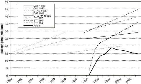
The important message we want to reiterate is that—no matter how good the data are—there will always be uncertainty. If we ignore uncertainty, our decision-making can be far off the mark. A classic example is the channel tunnel revenues projections, as documented by Marchau et al. (2019):
The planning for the Channel Tunnel provides an illustration of the danger of ignoring uncertainty. Figure 1.1 shows the forecasts from different studies and the actual number of passengers for the rail tunnel under the English Channel. The competition from low-cost air carriers and the price reactions by operators of ferries, among other factors, were not taken into account in most studies. This resulted in a significant overestimation of the tunnel’s revenues and market position (Anguara 2006) with devastating consequences for the project. Twenty years after its opening in 1994, it still did not carry the number of passengers that had been predicted. – (Marchau et al. 2019, 2)
There are basically three big sources of uncertainty to deal with: Model uncertainty, data quality, and residual uncertainty. We want tp briefly introduce them for two important reasons. For one, trying to get a handle on what you do not know or what you are uncertain about can be crucial. For another, your data collection efforts should naturally be geared towards where you can reduce uncertainty the most.
- Model uncertainty. Sometimes also called system uncertainty. We like the term model uncertainty because we want to include all the implicit mental models you might have—but never fully spelled out—about how the world works. All our (mental) models are simplifications, and sometimes we simplify away from something important. In the channel tunnel example, the planners did not consider important competitive dynamics for travel routes to and from England. Another way of saying the same thing is: There is always the possibility you are operating under wrong assumptions. Unknown unknowns reside here.
- Data quality. Say you have decided on one model like the one in Figure 2.10 (or maybe a few alternative models) of the revenue generation process for supermarkets. You have a model of what drives the number of customers per month and the average basket size they buy. Now, you need to start forecasting how these drivers will develop. These forecasts will be based on assumptions and extrapolations from data. The quality of the data will be an important (but far from the only) driver of how much you can trust these forecasts. Common statistical methods provide means of quantifying aspects of this uncertainty, and we will talk about this in more detail in Chapter 5. However, data quality has numerous facets, some hard to get a good handle on. Is data selected, censored, or missing in a non-random way, is current data even representative of the expected future dynamics, etc.?
- Residual uncertainty. This is the biggest and often most difficult to grasp the source of uncertainty. It arises from all the aspects of the problem we have either not included in the model or could not measure. Take a coin flip. It is, in principle, a well-understood physical mechanism. If we could measure all aspects of it, wind, angle, and force of the flip, etc., then we should be able to forecast quite accurately whether a coin lands heads or tails every time. However, even in this simple case, measuring all aspects of the problem without any measurement error is impossible. Thus, even here, there will always be residual uncertainty about how the coin will land. In real-world problems, it is common that certain dynamics are either too complicated (some competitive dynamics) to be forecast with any degree of precision or simply unknown to us. Thus, in many situations, it is impossible to quantify the residual uncertainty, and we have to think about how to make sensible decisions in these cases, too.8
A vast body of theory and literature hides behind and qualifies this simple answer. For example, both terms, utility and probability, are complex and challenging concepts. For those interested in a more thorough treatment Gilboa (2009) “Theory of Decision under Uncertainty” is a highly recommended introduction.↩︎
The following examples are inspired and heavily adapted examples from Chapter 1 in Gilboa (2009).↩︎
In a previous version, we had one additional step at the beginning: Detect the problem. Sometimes the problem is clear. Designing a new sales forecasting model or optimizing inventory are problems that are usually handed to you. However, sometimes we need to realize first that there is a problem (e.g., production quality is slowly decreasing). This does not always happen automatically. Well-designed monitoring systems that collect data and measure developments across multiple dimensions often throw the first warning signs that something needs to be looked at. (And somebody had to come up with the idea that it might be a sensible business precaution to install such a monitoring system.)↩︎
Again, disclaimer, these are simulated data↩︎
And if the relation between the variables is roughly linear. More on that in Chapter 5.↩︎
OLS minimizes the sum of squared errors, which means we care about mean values.↩︎
Some view causal analysis as distinct, some as very special and case of predictive analysis. See Gelman and Hill (2006), chapter 9.↩︎
There are interesting philosophical problems here that we don’t have the time to cover. For example, if we didn’t include competitive dynamics in our model, is this model uncertainty or residual uncertainty? It depends. If we are fairly certain that competition matters and simply could not include it, this is residual uncertainty. We think of a model to cover the relevant dynamics. For example, if competitive dynamics affect the relation between our main variables of interest, then we have a wrong model. If competitive dynamics only affect the main variable of interest but not others, then we might not necessarily have a bad model for the problem of interest.↩︎