4 Ratio Analysis
4.1 Purpose of this chapter
After having started to understand the business a firm is operating in and checked for accounting distortions, the time has come to analyze the firm’s performance. Ratios are an indispensable tool to do this. Ratios are the language used by analysts and management to discuss a company’s performance. We will also use them to construct forecasts and verify their plausibility.
An important piece of advice provided by our own teachers, Lundholm and Sloan, is that “Ratios do not provide answers, they just help direct you in your search for answers”. This is key, as we will see. Managers also know that investors sometimes fixate on certain ratios and sometimes window-dress accordingly (e.g., Lehman’s ‘Repo 105’). Thus, we always caution you not just to blindly trust ratios, but always to interrogate them.
There are different ratio systems, some of them industry-specific. We prefer to use the Advanced DuPont decomposition of \(ROE\). The Advanced DuPont decomposition is the cornerstone of many classic FSA textbooks (e.g., Penman 2012; Wahlen et al. 2017; Lundholm and Sloan 2019; Koller et al. 2020). We further believe the Advanced DuPont decomposition works well for tying ratios to different aspects of a firm’s business model. But, as always, this is not the only way of conducting a ratio analysis.
4.2 The enterprise value perspective
4.2.1 Separating operating from financing activities
Our starting point is, once again, our core value driver \(ROE\).
\[ ROE = \frac{\text{Earnings for the period}}{\text{Average equity during the period}} \]
Before proceeding further, notice the “average equity during the period” in the denominator. Net income is earned over a period (a flow), while common equity is measured at a point in time (a stock, i.e., a balance-sheet snapshot). We want to relate the flow to a representative level of the stock during the period. Using an average is the default approach.
Figure 4.1 illustrates this. The assumption is that equity changed gradually over the period in which net income was measured. As the bottom-left plot of Figure 4.1 shows, this does not have to be the case—for example, a large equity issuance could occur just before the fiscal year-end.

In this chapter, “operating” means “related to the core business” and is contrasted with “financing” (related to funding the business). This differs from Chapter 3, where “strategic” versus “operating” contrasted long-term vision with short-term execution.
Coming back to our starting point, \(ROE\). It shows how profitable the operations are in terms of return to the firm’s owners. We want to understand where this profitability comes from and will derive a ratio system that will guide us in this analysis. As we shall see now, there are three reasons for high profitability: efficient use of operating assets, pricing power and cost advantages, and leverage effects. We want a ratio system that disentangles these three aspects and helps us to analyze the determinants of all three determinants.
The first step towards this goal is to cleanly separate operating from financing items in the financial statements. Figure 4.2, adapted from Penman (2012) shows how investors generally think about a firm as it stands between capital markets and product markets.

We view the firm as collecting capital from capital markets—either from shareholders or debtholders. It uses this capital to invest in operations, as represented by net operating assets. The operations then exchange funds, goods, and services with the product markets. Funds leave the firm toward product markets as operating expenses (OE) and enter from customers as operating revenues (OR). The generated funds are ultimately returned to debtholders (F) and shareholders (d).
An important aspect highlighted in Figure 4.2 is the duality of net operating assets with capital invested from all capital providers. Contrast this with Figure 3.4, reproduced below in Figure 4.3:

Whereas in Figure 4.2 operations and financing of those operations are clearly separated, they are not on a standard balance sheet in Figure 4.3. We see financial assets on the asset side and operating liabilities on the liabilities side. A similar mixing can be seen on the income statement. If we really want to know what amount of capital is needed to fund the current operations, we need to restructure the balance sheet. And if we really want to know how profitable the operations are before disbursing funds to different stakeholders, then we need to restructure both the balance sheet and the income statement. As Figure 4.3 shows, we get there by:
- Classifying all balance sheet items as either operating or financing related.
- Doing the same with all income statement items, ensuring that the classification is consistent (e.g., if we classify certain investments as strategic and, therefore, operating, then the corresponding interest income on the income statement also needs to be classified as operating).
- Netting operating liabilities against operating assets to obtain net operating assets (NOA), and netting financial assets against financial liabilities to obtain net financial obligations (NFO).
- Separating net income into after-tax net operating income (\(NOI\)) and after tax net financial expense (\(NFE\)).
4.2.2 Leverage
Doing this separation well is crucial for right-sizing the magnitude of the investment in the actual operations of the company. It is also crucial for cleanly separating operating from financial effects.

Figure 4.4 shows why it is important to separate operating from financing effects. The left-hand side of Figure 4.4 shows a firm that is 100% equity financed and has $100 of capital invested in operations. Those operations earn a return-on-net-operating assets of 10%, which is $10.
Next, imagine that this firm has the opportunity to grow and expand its operation. It invests an additional $100 into operations, effectively doubling the size of operations. However, this time, the additional capital invested comes from debt. The profitability of the operations has not changed, despite the doubling in size (\(RNOA = 10\%\)), so it earns $20 now. The debt is financed at 5% so it needs to pay $5 in interest expense. Net income is now $20 − $5 = $15, so \(ROE\) = $15 / $100 = 15%—up from 10% in the all-equity case. \(ROE\), our anchor measure of value creation, is thus a mix of financing effects and operating profitability!
This is not an error; this is perfectly reasonable economics (one that leveraged buyouts have been exploiting for a long time). It is called the “leverage effect”. Because the interest rate of 5% is lower than the \(RNOA\), we can raise new capital cheaper compared to the return it generates when employed in the firm. The difference falls to equity holders, raising the \(ROE\)! While this is nice, when we want to analyze the actual profitability of the operations, we need to take out this leverage effect first. Otherwise, differences in capital structure will interfere with our assessment of the profitability of the operations. That is the purpose of the reformulation of the balance sheet and income statement into net operating assets, and so on.
An important implication is whether this leverage effect truly creates value. Recall from the residual income model that value depends on \((ROE_t - r) \cdot CE_{t-1}\) (see Equation 2.2). If leverage raises \(ROE\) but also raises the required return \(r\)—because equity becomes riskier—the net effect on value may be zero. This is the classic insight of Modigliani and Miller (1958). The empirical evidence is nuanced; interested readers may consult Graham and Leary (2011). We shall now return to the issue of cleanly reformulating the financial statements.
4.2.3 Details on reformulating the financials
We have the following categories to consider:
- Operating assets (OA): Assets tied to the operations of the firm
- Operating liabilities (OL): Liabilities arising from operations (e.g., accounts payable, deferred revenues, pension liabilities)
- Financial assets (FA): Not relevant for operations. Temporary stores of financing funds
- Financial obligations (FO): Representing external funding other than through equity. Also called ‘Financial Liabilities’
Rather than going through typical line items, we believe that it is best to talk about the intuition. Operating assets and liabilities are those that are used during the normal business of the firm. Financial assets are basically funds parked on the balance sheet. They are not needed for operations. While they might be converted into operating assets through investments in the future, they are not contributing right now to operations. Financing liabilities represent external funding of operations.
Classifying items on the balance sheet into operating or financing is mostly fairly obvious. If an item does not fit one category, it must be the other category. Cases like inventories or accounts payable are obviously integral to operations. In other cases, like pension liabilities, this is less obvious and sometimes handled differently by different analysts. In such cases, we find that it helps to think about both the asset and the corresponding income statement items together, which in this case is wage expense and related adjustments. If we view pensions as a form of compensating employees for their labor, then it is an operating activity. Some analysts prefer to classify pension liabilities as a form of financing liability, but this argument seems to us to only hold in special cases.
Other items that are less clear are deferred taxes and similarly related items and equity investments. In the first case, taxes are generally considered an operating expense (it is difficult to call it a financing activity). Intuitively, equity investments can be both a strategic investment or a medium-term position for parking funds till needed. It is a good example of items that might be classified differently depending on the firm. In each case, the corresponding interest income of the investment also must be classified in accordance with the balance sheet classification.
As a practical default, classify pension liabilities as operating (they compensate employees) and deferred tax liabilities as operating (taxes are a cost of doing business). Deviate from this default only when you have a clear economic reason for doing so.
Also note that there are often different ways to arrive at the same decomposition. Here are some examples:
- Net Financial Obligations (NFO): debt + preferred stock + minority interest − financial assets
- Net Operating Assets (NOA): invested capital = total assets − (total liabilities − NFO)
- Net Operating Assets (NOA): common equity + NFO
All of this is obvious once you understand the balance sheet in Figure 4.3. Preferred stock and minority interests are generally considered external financing from the point of view of common equity holders, which is the position we generally take. The minority interest reflects a small stake in consolidated subsidiaries that is not owned by common equity holders. Thus, they are classified as financial liabilities. Both preferred stock and minority interest reflect funds provided by parties other than common equity holders. Although it is not debt, it is still external from that point of view.
Once the balance sheet items are classified, the income statement classification usually follows. Again, there are different combinations, leading to the same answers:
- Net Operating Income (NOI): (EBIT + non-operating income) \(\cdot\) (1 − tax) + other income − extraordinary items + discontinued operations
- Net Operating Income (NOI): net income + net financing expense
- Tax: effective tax rate = (income tax expense)/(earnings before taxes)
- Net Financing Expense (NFE): interest expense \(\cdot\) (1-tax) + preferred dividends + minority interest in earnings
Again, the most important thing is consistent classification. E.g., the expenses of assets classified as operating should also be classified as operating.
4.3 The advanced DuPont decomposition
With the reformulation done, we can now proceed with our ratio analysis. To reiterate, the main purpose of the reformulation was to help us to disentangle operating from financing drivers of \(ROE\). We can see how this works using a simple expansion and rearranging of the \(ROE\) ratio, as shown in Equation 4.1. In the third line, we multiply and divide each term by the relevant balance sheet item—\(NOA\) for operating income and \(NFO\) for financing expense—to create recognizable ratios:
\[ \begin{aligned} ROE &= \frac{Net Income}{Equity}\\ &= \frac{NOI}{Equity}-\frac{NFE}{Equity}\\ &= \frac{NOI}{NOA}\cdot\frac{NOA}{Equity}-\frac{NFE}{NFO}\cdot\frac{NFO}{Equity}\\ &= RNOA\cdot\frac{NOA}{Equity}-(i\cdot(1-tax))\cdot\frac{NFO}{Equity}\\ &= RNOA\cdot\frac{Equity + NFO}{Equity}-(i\cdot(1-tax))\cdot\frac{NFO}{Equity}\\ &= RNOA\cdot\left(1+\frac{NFO}{Equity}\right)-(i\cdot(1-tax))\cdot\frac{NFO}{Equity}\\ &= RNOA+ \left(RNOA-i\cdot(1-tax)\right)\cdot\frac{NFO}{Equity}\\ &= RNOA+ Spread\cdot\frac{NFO}{Equity}\\ \end{aligned} \tag{4.1}\]
This decomposition is called the Advanced DuPont decomposition. The last line highlights the separation of operating and financing components of \(ROE\). Return-on-net-operating-assets (\(RNOA\)) is our measure of the profitability of operations. It is the return generated on the total capital invested in the firm. It is also sometimes called \(ROIC\) (return on invested capital) or return on capital employed. Note that definitions of ROIC vary across textbooks—some include goodwill, some exclude it. In this course, we define it strictly as \(NOI / NOA\). So \(ROE\), equals the profitability of operations plus a term that is the product of the spread between operating profitability and financing costs times financial leverage. The second part is the leverage effect we saw in Figure 4.4.
However, this is not where the ratio decomposition stops. We can further disaggregate \(RNOA\) into two important subcomponents by simply expanding sales.
\[ RNOA = \frac{NOI}{NOA} = \underbrace{\frac{NOI}{Sales}}_{\text{Net Operating Margin}} \cdot \underbrace{\frac{Sales}{NOA}}_{\text{Net Operating Asset Turnover}} \]
- NOI Margin: Margin left on each $ of sales after deducting all operating expenses. If not positive, firm will make losses no matter what
- NOA Turnover: How many $ of sales can be generated by $1 of NOA. Intuitive measure of operating efficiency
The decomposition of \(RNOA\) into efficiency of capital usage (NOA Turnover) and margin completes our search for the three components of profitability for shareholders: (1) efficient use of operating assets, (2) pricing power and cost advantages, and (3) leverage effects.
Margin and turnover are important aspects of a firm’s business model. Their multiplicative nature makes them substitutes. As Figure 4.5 shows, you can reach the same \(RNOA\) through high margin and low turnover or the reverse, low margin and high turnover.

Often, firms in the same industry arrange themselves in different areas of this trade-off. Some, for example, opt for a cost-leader strategy—reducing costs as much as possible and trying to use the existing capital as efficiently as possible (high sales to net operating assets). By cutting costs to a minimum, this strategy also implies limited investments in building a brand or other premium features that would warrant a price premium. Therefore, these strategies generally feature a low net operating margin. On the other side of the spectrum are product differentiation strategies. Many premium producers fall into this category. They feature a high price premium and thus a high net operating margin. At the same time, their production is usually more involved and requires a higher asset base for the operations, a longer inventory holding period, etc. As a result, net operating asset turnover is usually lower.
The three most common reasons driving the margin-turnover-trade-off are:
- Industry-wide production technology that requires significant capital investment
- Product differentiation versus a cost leadership strategy
- Vertical integration versus an outsourcing strategy
Understanding these dynamics—how business models map into ratios—is critical for a useful analysis of a firm’s current operating performance. Only this way can we also judge whether a firm’s business model is working well or not. A low margin might not be bad if the firm is aiming for a cost-leader strategy. Conversely, if a firm follows a product differentiation strategy, then seeing low margins is a sign that something is off with a key part of the strategy: sustaining a price premium.
Both operating margins and turnover are important for value creation. The role of efficient capital use, as captured by NOA turnover, is often forgotten. Recall Equation 2.5, where \(\gamma = CE / S\) was capital invested divided by sales—the inverse of turnover. In that formula, \(\Bar{g_s}\) is the expected long-run sales growth rate and \(\Bar{m} = (ROE - r)\) is expected long-run abnormal profitability. Turnover appears twice in this formula, because \(ROE\) is strongly affected by turnover:
\[ \begin{aligned} P_0 & = S_0 \cdot \gamma \left( 1 + \mathbb{E}_0\left[\Bar{g_s}\cdot \Bar{m}\right]\right) \\ & = S_0 \cdot \frac{CE}{S} \left( 1 + \mathbb{E}_0\left[\Bar{g_s}\cdot (\frac{S}{CE}\cdot \frac{NI}{S} - r)\right]\right) \end{aligned} \]
If capital turnover increases, the firm generates more sales per dollar of invested capital. The product \(S_0 \cdot \frac{CE}{S}\) stays constant because the increase in \(S\) cancels with the denominator. However, the higher turnover raises \(ROE\) through the \(RNOA\) channel, which increases the abnormal profitability term \(\Bar{m}\).
Due to the importance of margin and turnover for understanding how a firm creates value, we can—and should—drill even deeper (Figure 4.6). For margins, we look at different cost-to-sales ratios to understand the main drivers of margin development. Commonly encountered margins are the gross margin and the ‘earnings before interest and taxes’ (EBIT) margin. Here, we need to be careful. Sometimes, companies reclassify costs from one line item to another. There is often more information to be found in reports of listed companies. For example, a discussion of the time series of important margins is a required component of the MD&A in the US.

For turnover, the general approach is to see how frequently each operating asset and liability is ‘turned’ by dividing an appropriate measure of operating activity by the operating asset/liability. The measure of operating activity used is usually sales. (The cost of good sold is also often used for inventory. Purchases is often used for payables). An alternative approach to measuring turnover is to compute the average ‘days outstanding’: Take the reciprocal of the turnover ratio and multiply by the number of days in the period.
An important subpart of \(NOA\) turnover is working capital turnover, which is basically current operating assets (e.g., accounts receivable and inventories) minus current operating liabilities (mostly accounts payable and unearned revenues).1 It reflects the amount of short-term capital necessary to run the business. If a firm is not running as efficiently as it could, it is often one of the first things managers, consultants, private equity, etc. try to fix. The intuition is the same as with \(NOA\). For example, accounts payable are an important current operating liability. Accounts payable are open bills with suppliers and reflect goods and services received from suppliers that have not yet been paid. Those payables are similar to a loan. By agreeing to not being paid directly, the supplier “loans” the firm money until the due date for payment (incl. interest). Therefore, it reduces the amount of short-term liquidity necessary to run operations. Consider the following example.
Assume that accounts receivable are $100 at both the beginning and the end of the year
Assume that sales revenue is $1,200 for the year
Compute the accounts receivable turnover ratio:
$1,200 / (1/2 \(\cdot\) $100 + 1/2 \(\cdot\) $100) = 12
Compute the average number of days sales outstanding:
1/12 \(\cdot\) 365 days \(\approx\) 30 days
This means that customers take on average 30 days to pay. Stated differently, the firm extends credit to its customers for about 30 days. Because the firm has not yet received cash for these sales, the corresponding liquidity needs to come from other sources. Often a detailed analysis of the working capital components is a big part of the turnover analysis. An efficient collection of accounts receivables reduces the amount of capital investment necessary, a faster turning inventory does the same, etc.
A breakdown of further ratios commonly used for these detailed line item assessments can be found in the cheat sheet in this GitHub repository (github.com/hschuett/FSA-NotACheatSheet). We will not waste space replicating it here. Instead, we want to spend some time discussing the role of a good comparison.
4.4 Analyzing is comparing
Of course, whether an inventory is turning fast is relative. The inventory of a fast fashion retailer should turn faster than the inventory of a specialty chemicals producer. Such judgment calls generally involve some kind of comparison. Finding the right comparison in the right circumstances is often a critical step in any analysis. There are different types of comparison we can make.
- Comparing ratios over time for the same company
- Comparing ratios to those of companies in comparable situations and similar strategies (not necessarily competitors!)
- Comparing ratios to sensible theoretical benchmarks (e.g., \(ROE\) vs \(r\))
As an example, consider Table 4.1 with some advertising expense ratios. If you ever need to assess whether the amount of advertising spending is high or low, consider that Coca Cola spends roughly 10% for maintaining their brand as a benchmark.
The absolute figures are also important (e.g., roughly $4bn for investments into the Coca Cola brand. In fact, they might be more important; a ratio to sales might not be the best way to gauge the right level of advertising. For example, Apple does not break out advertising sales from its SGA expenses (selling, general, administrative), which are about 6-7% of sales. But Apples 2021 sales are $366bn and SGA is $22bn. Assuming that investments in the Apple brand are of similar magnitude as the Coca Cola brand investments, then a $4bn marketing budget would easily fit within those SGA numbers. (2015 was the last year Apple disclosed advertising expenses in the notes to the financial statements. Advertising expense was $1.8bn, $1.2bn and $1.1bn for 2015, 2014 and 2013, respectively on revenues of $234bn, $183bn, $170bn).
So, the right ratio and the right comparison depend on the situation and the question we are asking. You do not always need a ratio. Again, a solid grasp of accounting fundamentals and the underlying business makes it easier to find the right comparison (which is why it has its own Chapter 3). Otherwise, you cannot put the ratios into context. Industry expertise is key in properly analyzing ratios, but so is thinking carefully what drives the item that I want to analyze (in the example above, is the required investment in advertising really driven by sales?).
In addition, it is always helpful to know basic empirical patterns so as to know what to expect. As Figure 4.7 shows, mean reversion is generally also present in \(RNOA\) and in \(ROE\). \(RNOA\) is on average lower because its competitive benchmark is \(r_{wacc}\), the weighted average cost of capital, which is lower than the cost of equity. The latter incorporates the additional risk from leverage etc.

Figure 4.8 is intended to provide some general notion of plausible magnitudes of \(RNOA\) subcomponents. At the same time, it is intended to show you some more insights regarding sources of mean reversion. As you can see, gross margins (the top left plot) are surprisingly fixed over time and mostly above 25%. Net operating income margins, on the other hand, show some mean reversion and are mostly around 10%. This also tells us that most costs by companies are below cost-of-sales on the income statement. \(NOA\) turnover shows some clear signs of mean reversion for the top deciles and shows a wide range of magnitudes.

4.5 Conclusion
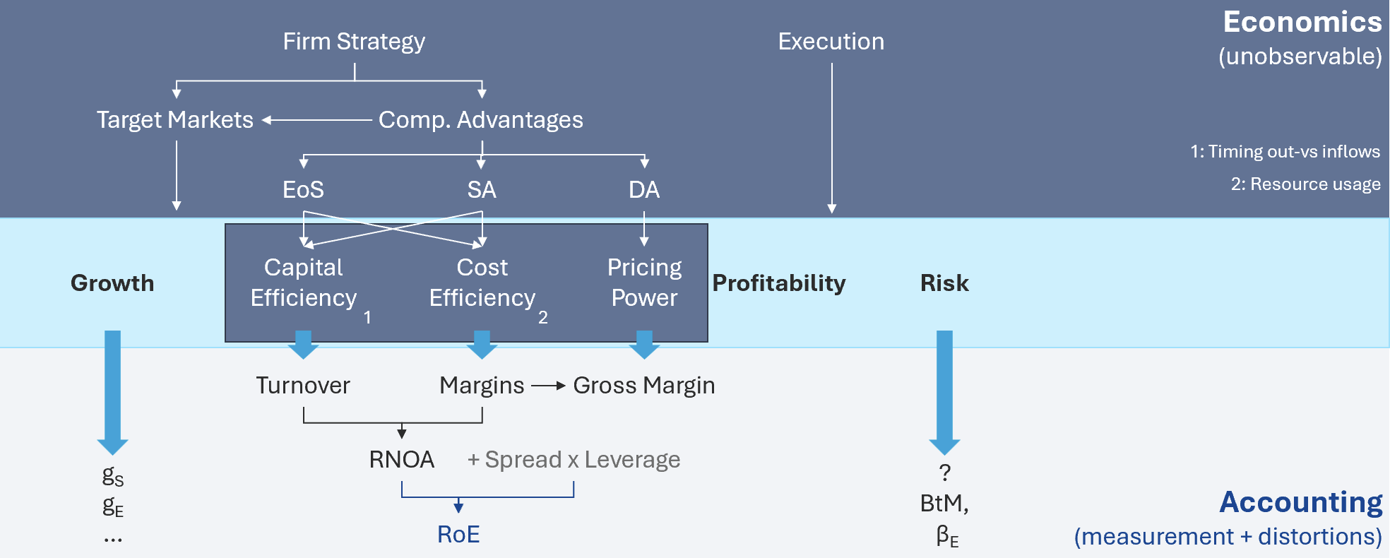
To summarize, this chapter introduced a top-down system of ratios aimed at analyzing the determinants of profitability. It decomposes \(ROE\) into three main sources of profitability: (1) efficient use of operating assets, (2) pricing power and cost advantages, and (3) leverage effects. Then it drills further into possible main drivers of each of the 3 cases. We discussed how ratios tell us what business model a firm is following and whether it works well. Figure 4.9 summarizes this rationale. The economics of a firm are driven by management’s strategy and execution. It involves two main decisions: a) which markets does the firm want to operate in and b) what are the ways in which it wants to ‘win’ in those markets (i.e., what competitive advantages does it want to cultivate? Economies of scales, supply, or demand advantages?). Those advantages, among other things, should transalte into either higher capital efficiency, cost efficiency, or pricing power than the competition. Neither of the three aspects is directly observable. Accounting can inform about all three, but one should never forget that accounting is a measurement system that relies on estimates and sometimes does not capture all of the firm’s resources or mismeasures resource usage. What we discussed in this chapter is how we can use ratio frameworks like the advanced dupont decomposition to compute ratios follows exactly this logic and can help us asses the key components of a firm’s strategy in a structured and principled way.
We also discussed how important the right comparison is for interpreting a ratio. For this, we need the right data, which is the topic of the next chapter.
4.6 References
Current means “to be expected to be liquidated within 12 months or during the operating cycle.” Working capital is not always defined consistently. But the intuition is that it is the current portion of \(NOA\).↩︎
Disney: “increase in advertising expense for fiscal 2021 compared to fiscal 2020 was due to higher spend for our DTC streaming services. The increase in advertising expenses for fiscal 2020 compared to fiscal 2019 was primarily due to the consolidation of TFCF and Hulu, partially offset by lower advertising for our theatrical, home entertainment and parks and experiences businesses.↩︎
Apple’s advertising expense was $1.8bn, $1.2bn and $1.1bn for 2015, 2014 and 2013, respectively on revenues of $234bn, $183bn, $170bn↩︎