6 Forecasting

6.1 Purpose of this chapter

All the steps discussed so far are preparation steps for the eventual task of building forecasts. In this chapter, we will go through the whole process of building a set of forecasts. By the end you will hopefully have a good grasp on what the key ingredients to a well-structured spreadsheet model are that contain a robust and defendable set of forecasts.

6.2 Setting up the model

Our financial model needs to be set up to support our final valuation model. To value the company, we need to forecast our core value drivers into the future, up to infinity (Equation 6.1).

\[ P_0 = CE_0+ \mathbb{E}_0\left[\sum^\infty_{t=1}{\frac{NI_{t}-r \cdot CE_{t-1}}{(1+r)^t}} \right] \tag{6.1}\]

Of course, we cannot make infinitely many forecasts. That issue is easily sidestepped by assuming that the firm’s residual income ($NI_{t}-r \cdot CE_{t-1}$) grows at a constant rate after a so-called terminal value period $T$:

\[ P_0 = CE_0+ \mathbb{E}_0\left[\sum^T_{t=1}{\frac{(RoE_{t}-r) \cdot CE_{t-1}}{(1+r)^t}} + \frac{(RoE_{\infty}-r) \cdot CE_{T}}{(1 + r)^T \cdot (r - g_\infty)} \right] \tag{6.2}\]

According to Equation 6.2, what we want to do is to construct pro-forma financial statements up to T years into the future, so that we can derive $ROE$ and $CE$ forecasts from it. These statements also give us the option to derive free cash flows for a DCF valuation model (or inputs to whatever other model we want to use to communicate the final valuation). Even if we later use a DCF model for communication purposes, we like to have a RIM model in the back as a sanity-check option. The financial statements are crucial to sanity-check our forecasts in any case.

We will discuss in more detail how to set the length of the detailed forecast horizon (whether $T$ is five, ten, or twenty years in the future). We will do so in Section 6.5. Likewise, after period $T$, we need a forecast for the terminal $ROE$ and growth rate $g_\infty$. The choices for both are strongly governed by economic theory, which we discuss in more detail in Section 6.6.

In all likelihood your model will be contained in an excel workbook, so let us talk about a proper setup of such a workbook. In our experience, many firms have some kind of explicit or implicit policy on how to set up Excel files containing a financial model + valuation model. Here are what we consider to be common practices.

Separate data input from modeling. Have one worksheet for raw historical data. Financial statements, footnote data, external report data, etc. Ideally, you have something like 5 years of past historical data. But you can go back further if you think stale data from, say 10 years ago, can still be informative about today’s business cycles, etc. Some like to have a spreadsheet per data source, and others prefer to have all raw data in one giant spread sheet. The right answer probably depends on the amount of raw data that you feed into your model. The important part is to have the raw data input separate from any calculations
Have one sheet with integrated financial statements, income statement, balance sheet, and cash flow statement. Build them close to what the firm reports and at the level of detail you need. It will contain not only the historical statements (fed from the raw input sheet) but also your forecasts of future statements. Having it follow the firm’s own format is important for benchmarking, especially if you are an analyst and new financials come out. You want to be able to quickly compare the company numbers with your own.
Have one sheet dedicated for cost of capital computations. For example, containing market data and $WACC$ calculations, if this is how you choose to model the cost of capital (more on that in Chapter 7).
Have one sheet for reformulated pro-forma statements. Here, the reformulation of the operating and financial assets and liabilities happens. Also, all adjustments for accounting distortions are applied here. This forms the basis for your ratio analysis
Have one sheet with the timeline of the advanced Dupont decomposition and any ratios you need to forecast the balance sheet. Forecasts of core value drivers and its components ($ROE$, $RNOA$, etc.) should be clearly visible. You want to minimize user input into ideally only this sheet and maybe 1-2 more detailed forecasting sheets like a sales forecasting sheet.
Have a valuation summary sheet that contains the RIM and any other valuation model you want to produce.

Models structured like this are very common in the industry. Well-built models nearly always cleanly separate data from automatic calculations from user input. Of course, well-built models are also clear to read and not a maze of formulas where you have to hunt from one cell to the next to figure out where a weird-looking ROE estimate is coming from. With a set-up like this we are prepared to finally start forecasting.

6.3 Structured forecasting

6.3.1 Structure of a forecast

Figure 6.1 shows a typical forecasting procedure. We start by forecasting sales. Since many of the following forecasts implicitly or explicitly will depend on sales forecasts, the sales forecast is in many respects the most crucial one. Next, we use our understanding of operating margin drivers to forecast the operating part of the income statement and our understanding of operating efficiency (turnover) to forecast the balance sheet. There are some interdependencies here (like depreciation). But often it helps to start with the margin/income statement side. Afterwards, we forecast leverage, which basically amounts to forecasts of capital structure. This is often a question of a sensible forecast of where the funding for the forecasted growth and investments is supposed to come from. This determines financial expenses. The only thing that is left is a forecast of the tax rates and then you can complete the income statement and balance sheet forecasts. Once you have those, the cash flow statement forecasts follow mechanically.

flowchart TD
    SALES["Forecast Sales"]
    MARGINS["Forecast Operating<br>Margins"]
    TURNOVER["Forecast Turnover"]
    DEPR["Depreciation"]
    OPEX["Operating Expenses"]
    FINEXP["Financial Expenses"]
    TAX["Tax Expense"]
    OA["Operating Assets<br>+ Liabilities"]
    LEV["Forecast Leverage"]
    FL["Financial Liabilities<br>(+Assets)"]
    IS["Income Statement"]
    BS["Balance Sheet"]
    CF["Cash Flow Statement"]

    SALES --> MARGINS
    SALES --> TURNOVER
    MARGINS --> OPEX
    TURNOVER --> OA
    OA --> DEPR
    DEPR --> OPEX
    OA --> LEV
    LEV --> FL
    FL --> FINEXP
    FINEXP --> TAX
    OPEX --> TAX
    TAX --> IS
    FL --> BS
    IS --> CF
    BS --> CF

    style SALES fill:#e8d8b8,stroke:#333
    style MARGINS fill:#e8d8b8,stroke:#333
    style TURNOVER fill:#e8d8b8,stroke:#333
    style DEPR fill:#e8d8b8,stroke:#333
    style LEV fill:#e8d8b8,stroke:#333
    style IS fill:#003366,stroke:#003366,color:#fff
    style BS fill:#003366,stroke:#003366,color:#fff
    style CF fill:#003366,stroke:#003366,color:#fff

Figure 6.1: Source: Figure 7.1 ‘A Systematic Forecasting Framework’ by Lundholm and Sloan (2019)

6.3.2 Forecasting sales

Sales are typically forecast using a top-down approach (starting with market size) or a bottom-up approach (thinking about the number of customers that can be serviced). Both are shown in Figure 6.2.

Figure 6.2: Typical Sales Forecasting model build-ups

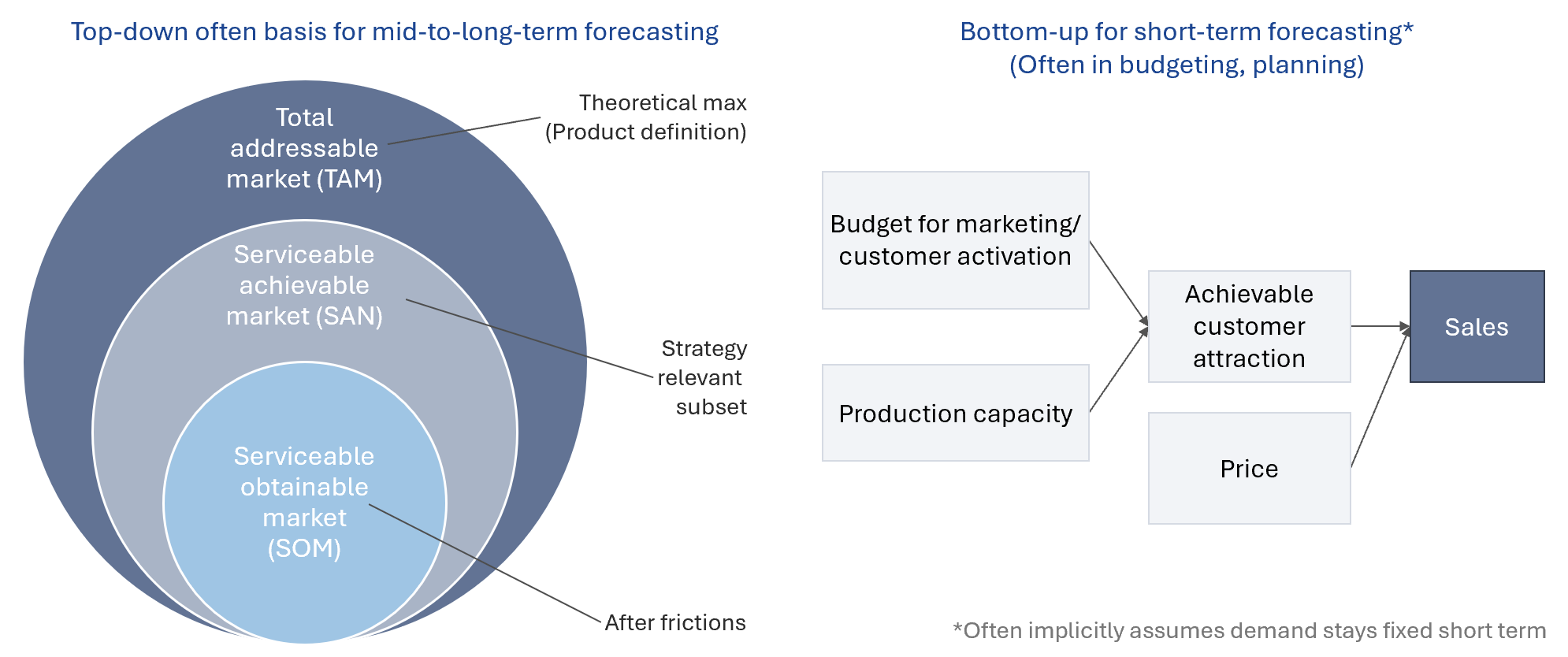
The top-down approach uses a simple decomposition of sales into $\text{Sales}_t = \text{Market Size}_t \times \text{Market Share}_t \times \text{Price}_t$. We start by sizing the total addressable market, then restricting the market size to the part actually serviceable, and then we try to forecast market share. Together, this equals volume, which multiplied by price equals sales. If the firm is in multiple markets (different products, services, or distinct regions), we want to forecast each of these markets separately, in as much detail as high-quality data allows us to do so.

The top-down approach is useful when it is easy to reason and collect data on the size of the market and market shares. It is also bound to be reasonably precise if the market is mature and grows slowly, because then historical data is a good basis (and, in turn, third-party forecasts of market developments are usually not too terrible). In these situations, analysts (given their time constraints) often use reliable third-party forecasts of market growth and focus their own efforts on getting market share and other parts of the forecasts right. This makes perfect sense, but we still want to warn you not to just take any market forecast you can find on the internet. There are many bad market forecasts out there, even from decent forecast providers. Always try to ensure that your most crucial forecast building blocks rest on sound data and confirm with your own reading of market dynamics.

In the short run, company guidance and projections can provide a good anchor for your forecasts (but remember the Peloton example from Chapter 5; companies can also be wrong). For forecasts further out, strategic considerations become the main forces you should think about. Which company is best positioned for long-term success in this market? Who has the clearest competitive advantages and should thus win out in the long run? Are there products or services on the horizon that might displace the current ones? And so on.

Surprisingly, the top-down approach is often used and helpful for new product markets. But in this case, it requires much more work to be useful, not just guesswork. Given the lack of history, it is tough to estimate the market size and market growth (speed of penetration) of new products. As always, finding good comparisons can be the crucial piece in reasoning (recall Section 5.3). Forecasting—even machine-learning-based forecasting—is nothing but identifying similar situations in history and assuming that something similar will happen again. Are there mature products whose history can serve as a good benchmark? Imagine that you had to size the potential market for smart home gym equipment. Can you get data on traditional home equipment as a benchmark? If so, would smart home equipment, due to its greater functionality, be adopted faster or maybe slower (higher prices?). You may also have to think about changes in preferences during the Covid pandemic. Again, finding a good comparison to help motivate the amount of adjustment is important.

Forecasting market share and price point is even more difficult than forecasting market size. You need to have a good idea of competitors’ offerings and competitive advantages to determine price points and likely market shares. We will repeat this like a mantra for most of the rest of the chapter: Finding a similar competitive situation in recent history from which one can extrapolate decent predictions of competitive developments is the best you can do here. The analysis also needs to draw on our previous analysis of cost structures and operating efficiency. The choices made here will be important for the forecasts of expenses and balance sheet items as well.

In contrast to the market-based top-down approach, the bottom-up approach relies on projections of customer demand. It is most often used in budgeting decisions where budget and capacity are often fixed. For these decisions, the forecasting task is better described as: “What sales are achievable with our current assets and budget” We believe this is mostly useful for short-term forecasts, where you have data on the customer base, customer turnover, and have a decent model of the strategy to acquire new customers.

Top-down, bottom-up, or a mixture of both; we forecast sales for next year $t+1$, $t+2$, until $T$. By the nature of the subject, the further out into the future our forecast of sales, the more they will be wrong. Markets, especially new ones, are governed by too many dynamics that change for reasons you could not have anticipated. Thus, it is important to make forecasts that are consistent with common industry dynamics and plausible growth trajectories based on historical experience. Due to the integral nature of sales forecasts to the rest of your model, it is also crucial to perform a sensitivity test on your sales forecasts. Do your forecasts change significantly when changing key assumptions?

6.3.3 Forecasting expenses

When turning to forecasting operating expenses—and really the rest of the financial statements—, we draw on all the insights gathered from your previous analysis of the past. we should already have a decent understanding of the economic relationships driving each line item and have an idea how to map forecasts of these dynamics into the right ratios (remember our discussion from Chapter 4 about whether judging the amount of marketing spend relative to sales is always a good idea). What is left is to forecast how the economic relationships are going to develop and forecast these ratios accordingly. Let yourself be guided by historical values of each ratio. Start with the value of the previous year and adjust accordingly. For example, if you believe that a company will experience improvements in production technology via learning effects and the company is not yet facing such competition as to have to pass these cost efficiencies over to customers via lower prices, then you would expect the cogs/sales ratio to decrease (cost-of-sales divided by sales). You forecast such an improvement based on similar learning effects in comparable cases. You multiply it by your sales forecast and arrive at your cost of sales forecast. Do this for every important line item. Think about the economics that govern the line item. Thinking in ratios often helps, but you should also look at the raw numbers as a sanity-check. If the line item is not crucially important in terms of % of sales and you cannot get a good rationale of a forecast, using last year’s ratio as a last resort is common practice.

A special case is depreciation. First, depreciation is not always broken out as a separate line item by firms. It is sometimes part of cogs and part of sga. In many cases, the notes to the statements tell you more details to figure this out, but it is not guaranteed, especially for small firms. Depreciation is usually best forecast as a percentage of PPE and not sales. It is still partly sales dependent, since PPE turnover is often used to forecast PPE needs. However, in practice, depreciation is usually modeled using either gross PPE or net PPE. Assuming straight-line depreciation, depreciation is just gross PPE divided by the useful life of the asset. So, you need to get the useful life right and make sure you properly account for asset retirements. If you use net PPE, there are some guiding benchmarks. In steady state, the ratio of depreciation to net PPE should be $\approx 1/(0.5 \times \text{useful life})$. You can see this also in Figure 3.6 in the section on accounting distortions. This is because in steady state, where depreciation roughly equals new investments, the PPE is on average roughly half-way through their useful life. For growing firms, it should be lower because the existing assets are less than half-way through their useful life. Even for those firms $1/(0.5 \times \text{useful life})$ is a useful guiding ratio, since it is the ratio that depreciation to average net PPE should converge to once the firm matures. The difficult part is to get an estimate of the useful life of the assets. If the notes to the financial statements are not informative, you have to make educated guesses based on comparable assets from other companies.

Finally, tax expenses are often difficult but important. Some prefer to use pre-tax earnings times an estimate of effective tax rates, some split up the computation into a calculation of operating taxes via EBIT (EBITA in Koller, Goedhart, and Wessels (2020)) and adjust for taxes related to non-operating accounts. The reason is that applying the effective tax rate to non-operating items, like interest expense and income, makes the RNOA and free cash flow forecasts change as leverage and non-operating income changes. The remedy is to apply the forecast of the effect tax rate to $NOI$ and a marginal tax rate (if not available, the statutory tax rate) to the remaining pre-tax items (Koller, Goedhart, and Wessels 2020, 272). The effective tax rate often differs from the statutory one due to tax credits and similar advantages. For listed firms (US GAAP and IFRS) there are usually designated tax footnotes that explain that difference. Of particular importance are permanent differences. It is worthwhile to browse this note and look for things that might change in the future. Even if we decided to extrapolate the historical effective tax rate, we need to realize that any operating credits and incentives are then assumed to grow in line with EBIT. If we are not willing to assume this, we need to adjust.

6.3.4 Forecasting the balance sheet

We usually forecast components of net operating assets as percentage of sales (maybe with the exception of some working capital items like inventories and payables, which we could link to cost-of-goods-sold instead). Net financial obligations are often easier to forecast as a percent of total assets—or net operating assets. Financial obligations are driven by the capital structure of the firm; therefore, it makes more sense to first forecast the amount of net operating assets needed and then forecast what portion of $NOA$ (or total assets) is financed by debt.

Let us dig a bit deeper into the forecasts of net operating assets. In general, working capital forecast assumptions are a statement about a firm’s day-to-day operating efficiency. Your analysis of past operating efficiency ratios using appropriate benchmarks should be the foundation for these forecasts. In contrast, assumptions about the non-current part of net operating assets reflect your assumptions about the necessity of investments providing long-term future benefits (most notably, PPE and sometimes the development portion of R&D). Economies of scale on the balance sheet will be most visible in these long-run investments.

We typically forecast all balance sheet items except one called the “plug”: usually cash, debt, or equity. This one is left as the residual and is equal to the amount that is needed to make the balance sheet balance after we have forecast all the other items. There are many different opinions on what the best plug is. Ultimately, we do not think it matters much. We have to forecast two of the three (cash, debt, equity) and by doing so the third is an implicit forecast. We like to use retained equity, but that is just personal preference. The important thing is that you need to realize that you need to examine the plug forecast as much as all the others. And choosing one plug does not exempt you from making a capital structure forecast. For example, you might think that using debt as a plug might mean you don’t need to explicitly forecast the capital structure. But you do, at least implicitly, by then needing to forecast dividends and stock issuances, with the rest of the needed funds implicitly assumed to come from debt—you will always forecast a capital structure, either implicitly or explicitly.

We could spend much more time discussing individual line item forecasts on the income statement and balance sheet. However, there are many good tips and suggestions for forecasting individual line items provided in Lundholm and Sloan (2019) and Koller, Goedhart, and Wessels (2020). Rather than just repeating those here again, we prefer to refer you to these excellent sources. Instead, we will discuss in more detail the final two crucial aspects of forecasting: choosing the forecast horizon and dealing with terminal period assumptions.

6.4 Slight tangent: connecting the dots to other lectures

If you have taken a corporate finance class or other courses centered on cash flows more narrowly before, you might have come across the following way of forecasting free cash flows for your valuation model. First, forecast sales, then forecast a margin that gives you after-tax EBIT or NOPLAT, then forecast a reinvestment rate. That is a perfectly appropriate way to generate inputs to a valuation model. However, to get good forecasts of free cash flows, you still need to do what we advised above. The following nice example is from the blog of the well-known valuation expert Damodaran (The Sharing Economy come home: The IPO of Airbnb!):

Table 6.1: AirBnB forecast example from: The Sharing Economy come home: The IPO of Airbnb!. Values in thousands.

	Gross Bookings	Revenues	Op. Margin	EBIT (1-t)	Sales/Capital	Reinvestment	FCFF
1	$37,089	$4,692	-10.0%	($469)	2	$533	($1,002)
2	$46,361	$5,990	-3.0%	($180)	2	$649	($829)
3	$57,951	$7,565	0.5%	$38	2	$788	($750)
4	$72,439	$9,555	4.0%	$382	2	$995	($612)
5	$90,548	$12,066	7.5%	$778	2	$1,255	($478)
6	$109,020	$14,674	9.5%	$1,048	2	$1,304	($256)
7	$126,245	$17,163	13.4%	$1,724	2	$1,244	$479
8	$140,385	$19,275	17.3%	$2,495	2	$1,056	$1,439
9	$149,650	$20,749	21.1%	$3,288	2	$737	$2,551
10	$152,643	$21,370	25.0%	$4,007	2	$311	$3,696
TY	$155,696	$21,797	25.0%	$4,087	2	$817	$3,270

Note that Table 6.1 looks much simpler, but it actually follows the same idea we laid out before.

Start with revenue forecasts
Forecast (net) operating margins (the EBIT (1-t) here is equivalent to our NOI)
Decide on a sales to capital ratio. This is our NOA turnover! It is needed to compute the reinvestment needed to grow free cash flows because it dictates what capital investment is needed and thus what amount of cash needs to be spent on reinvestments.
Compute the free cash flow to the firm (to entity) as EBIT (1-t) minus reinvestments.
The capital invested and the implied ROIC follow from the previous numbers.

The take away from this short intermezzo is: Even if you learned this way of computing free cash flows for a valuation model, note that to get there, you ideally use the same principles of structured forecasting to arrive at your inputs. Turnover and margins are just as important to get decent free cash flow forecasts as they are to get decent earnings forecasts.

6.5 Forecast horizon

The choice of forecast horizon can have a huge impact on the final valuation of the firm. Examine Figure 6.3. These different mean reversion trajectories (no matter whether it is for sales, $RNOA$, or $ROE$) have very different valuation implications. Some have a more years of high growth (profitability) and then rapidly revert, some revert faster, some take longer to revert, and so on. We will treat the forecast horizon $T$ in Equation 6.2 as an explicit forecast horizon for how long it takes the firm to reach a steady state in which growth has tapered down to the average growth of the economy and profitability has reverted to its long-run value, usually $ROE = r$.

Figure 6.3: Different mean reversion trajectories

This might sound abstract and unrealistic. But the rationale for treating a firm as converging to average growth and no value creation is based as much on historic experience as—frankly—pragmatism. It is important to remind ourselves that we are tasked with forecasting how the firm will perform assuming that the firm will exist forever. Infinity is a long time and there is no way to make a sensible forecast for an infinite period. But, in our history, all important companies over the last centuries have returned to mediocrity or stopped existing. It is always tempting to think “this time it is different” (i.e., Google), but history so far tells another story.

Figure 6.4: Most valuable companies and sectors by era

Figure 6.4 shows for example that the most valuable company (by far) in the US in 1917 was U.S. Steel and the most important industries were Oil & Gas as well as Mining. After 100 years, U.S. Steel is a far cry away from its former glory, wrestling with at best average performance in a sector not nearly as crucial as before. The same can be said about IBM and AT&T, the most valuable companies in the 70s already. The message that this comparison hopefully conveys is that infinity is a long time, not only for companies but also whole sectors. Every hot sector in history has fallen out of favor eventually. Every company has either been caught by competition eventually or had to face a sector shift that stinted its markets. This experience is the justification for our forecasting approach. So far, every company in the history of the world has faced this fate. Why would we assume anything else? The only question is how long it takes for the firm to get there.

The appropriate forecast horizon depends on what we consider the market prospects to be. At what stage is the market of the firm and how large is its eventual size when mature? A second important consideration is how long it will take competition to force growth and profitability prospects to equilibrium. These considerations are captured together with some recommended time horizons in Figure 6.5. Five to ten years is the usual range, but some suggest 10-20 years. Consider Figure 6.5 only as a rough guide. Your own market analysis should guide this decision.

// Configuration for the forecast horizon matrix
horizonCfg = ({
  w: 720,
  h: 340,
  margin: { top: 50, right: 20, bottom: 20, left: 160 },
  colors: {
    cell:     "rgba(204, 153, 51, 0.25)",
    header:   "#003366",
    headerBg: "rgba(0, 51, 102, 0.85)",
    sideBg:   "rgba(0, 51, 102, 0.15)",
    stroke:   "#003366",
    text:     "#2c2c2c"
  }
})

horizonDiagram = {
  const svg = d3.create("svg")
    .attr("viewBox", `0 0 ${horizonCfg.w} ${horizonCfg.h}`)
    .attr("width", "100%")
    .attr("height", "auto")
    .style("font-family", "'IBM Plex Sans', 'Helvetica Neue', sans-serif");

  const g = svg.append("g")
    .attr("transform", `translate(${horizonCfg.margin.left},${horizonCfg.margin.top})`);

  const cols = ["Low\n(mature)", "Medium\n(consolidating)", "High\n(start-up)"];
  const rows = ["None", "Yes, but only\nshort run", "Yes, and for\nlonger run"];
  const values = [
    ["2 years", "5 years", "10 years"],
    ["5 years", "5 years", "10 years"],
    ["10 years", "10 years", "10–20 years"]
  ];

  const cellW = 150, cellH = 60;
  const plotW = cols.length * cellW;
  const plotH = rows.length * cellH;

  // Column header bar
  g.append("rect")
    .attr("x", 0).attr("y", -40)
    .attr("width", plotW).attr("height", 30)
    .attr("fill", horizonCfg.colors.headerBg).attr("rx", 3);
  g.append("text")
    .attr("x", plotW / 2).attr("y", -20)
    .attr("text-anchor", "middle").attr("font-size", 13)
    .attr("fill", "#fff").attr("font-weight", 600)
    .text("Market-wide growth prospects");

  // Column headers
  cols.forEach((col, ci) => {
    const lines = col.split("\n");
    lines.forEach((line, li) => {
      g.append("text")
        .attr("x", ci * cellW + cellW / 2).attr("y", li * 14)
        .attr("text-anchor", "middle").attr("font-size", 12)
        .attr("fill", horizonCfg.colors.text)
        .text(line);
    });
  });

  // Row header background
  g.append("rect")
    .attr("x", -horizonCfg.margin.left + 10).attr("y", 20)
    .attr("width", horizonCfg.margin.left - 20).attr("height", plotH)
    .attr("fill", horizonCfg.colors.sideBg).attr("rx", 3);

  // Row header label (rotated)
  g.append("text")
    .attr("transform", `translate(${-horizonCfg.margin.left + 22},${20 + plotH / 2}) rotate(-90)`)
    .attr("text-anchor", "middle").attr("font-size", 12)
    .attr("fill", horizonCfg.colors.text)
    .text("Firm-specific competitive advantage");

  // Row headers
  rows.forEach((row, ri) => {
    const lines = row.split("\n");
    const cy = 20 + ri * cellH + cellH / 2;
    lines.forEach((line, li) => {
      g.append("text")
        .attr("x", -20).attr("y", cy + li * 14 - ((lines.length - 1) * 7))
        .attr("text-anchor", "end").attr("font-size", 12)
        .attr("fill", horizonCfg.colors.text)
        .text(line);
    });
  });

  // Cells
  rows.forEach((_, ri) => {
    cols.forEach((_, ci) => {
      const cx = ci * cellW;
      const cy = 20 + ri * cellH;
      g.append("rect")
        .attr("x", cx + 5).attr("y", cy + 5)
        .attr("width", cellW - 10).attr("height", cellH - 10)
        .attr("fill", horizonCfg.colors.cell).attr("rx", 4);
      g.append("text")
        .attr("x", cx + cellW / 2).attr("y", cy + cellH / 2 + 4)
        .attr("text-anchor", "middle").attr("font-size", 13)
        .attr("fill", horizonCfg.colors.text).attr("font-weight", 500)
        .text(values[ri][ci]);
    });
  });

  return svg.node();
}

Figure 6.5: Choosing an appropriate forecast horizon

6.6 Disciplining the terminal value

The rationale for choosing the forecast horizon period should have also made you aware that, generally speaking, short-run forecasts are driven to a larger extent by firm-specific considerations and medium-term to long-term forecasts by industry and macro dynamics. The terminal period assumptions are purely driven by macro considerations.

After period $T$, the firm is forecast to grow at a constant rate and have a constant profitability level. The present value of all the periods following after $T$ is called the terminal value. Since everything is constant, it is easy to compute (see Equation 6.2). Thus, there are two final choices to make: The terminal growth rate and terminal $ROE$.

There is a clear limit to the terminal growth rate as illustrated in Figure 6.6. Remember that when we talk about the terminal growth rate, we are talking about the growth rate applied to every year into infinity. If this rate is higher than the long run possible growth rate of the world, we effectively assume that the firm is eventually going to swallow the universe.

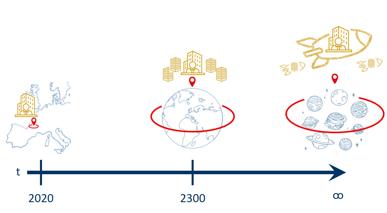
Figure 6.6: Terminal sales growth rate should not exceed the terminal forecast of GDP growth rate

For this reason, your terminal sales growth should not be higher than what an infinite GDP growth rate can be for the universe. Paraphrasing economic growth theory, the main drivers of economic growth are input factor growth and the rate technological advance. Average long-term GDP growth should converge to the rate of technological advance. That only helps us in as much as we can put a number on this. Unfortunately, that is tough. Usually a number between 3-5% is used. Sometimes, you also hear arguments to base the terminal growth rate on inflation and similar factors. However, inflation is itself driven by technological advance as famously advocated by former Federal Reserve Chairman Alan Greenspan.

“The past decade of low inflation and solid economic growth … is attributable to the remarkable confluence of innovations that spawned new computer, telecommunication, and networking technologies, which … have elevated the growth of productivity, suppressed unit labor costs, and helped to contain inflationary pressures”

— Greenspan A: Globalization. Speech, New York. 10 Mar 2005

The other terminal period assumption, terminal $ROE$, is also driven purely by economics. As long as you have no robust argument for why a firm should have insurmountable competitive advantages that will protect it from competition forever and ever, you should set the terminal period $ROE = r$ after adjusting for accounting distortions. The reported $ROE$ can be higher (because intangibles are missing from the books, etc.) But after adjusting for accounting distortions, $ROE$ should be equal to the cost of equity capital.

In summary, forecasting is again a task of finding good comparables and understanding the firm’s business and accounting well. Importantly, after you have arrived at a full forecast, we are not done! We need to check its plausibility using the pro-forma financial statements derived from our forecasts. Are the financial ratios sensible, are the statements plausible? (e.g., if you have a profitable firm and equity turns negative after three periods, something went wrong in your assumptions about fund usage). It is crucially important to sanity-check your forecasts.

6.7 References

Koller, Tim, Marc Goedhart, and David Wessels. 2020. Valuation: Measuring and Managing the Value of Companies. 7th Edition. John Wiley; Sons.

Lundholm, Russel, and Richard G Sloan. 2019. Equity Valuation and Analysis. 5th Edition. Independently published.